SimRank is a general similarity measure, based on a simple and intuitive graph-theoretic model. SimRank is applicable in any domain with object-to-object relationships, that measures similarity of the structural context in which objects occur, based on their relationships with other objects. Effectively, SimRank is a measure that says "two objects are considered to be similar if they are referenced by similar objects." Although SimRank is widely adopted, it may output unreasonable similarity scores which are influenced by different factors, and can be solved in several ways, such as introducing an evidence weight factor,[1] inserting additional terms that are neglected by SimRank[2] or using PageRank-based alternatives.[3]
Various aspects of objects can be used to determine similarity, usually depending on the domain and the appropriate definition of similarity for that domain. In a document corpus, matching text may be used, and for collaborative filtering, similar users may be identified by common preferences. SimRank is a general approach that exploits the object-to-object relationships found in many domains of interest. On the Web, for example, two pages are related if there are hyperlinks between them. A similar approach can be applied to scientific papers and their citations, or to any other document corpus with cross-reference information. In the case of recommender systems, a user’s preference for an item constitutes a relationship between the user and the item. Such domains are naturally modeled as graphs, with nodes representing objects and edges representing relationships.
The intuition behind the SimRank algorithm is that, in many domains, similar objects are referenced by similar objects. More precisely, objects and are considered to be similar if they are pointed from objects and , respectively, and and are themselves similar. The base case is that objects are maximally similar to themselves .[4]
It is important to note that SimRank is a general algorithm that determines only the similarity of structural context. SimRank applies to any domain where there are enough relevant relationships between objects to base at least some notion of similarity on relationships. Obviously, similarity of other domain-specific aspects are important as well; these can — and should be combined with relational structural-context similarity for an overall similarity measure. For example, for Web pages SimRank can be combined with traditional textual similarity; the same idea applies to scientific papers or other document corpora. For recommendation systems, there may be built-in known similarities between items (e.g., both computers, both clothing, etc.), as well as similarities between users (e.g., same gender, same spending level). Again, these similarities can be combined with the similarity scores that are computed based on preference patterns, in order to produce an overall similarity measure.
Basic SimRank equation
For a node in a directed graph, we denote by and the set of in-neighbors and out-neighbors of , respectively. Individual in-neighbors are denoted as , for , and individual out-neighbors are denoted as , for .
Let us denote the similarity between objects and by . Following the earlier motivation, a recursive equation is written for . If then is defined to be . Otherwise,
where is a constant between and . A slight technicality here is that either or may not have any in-neighbors. Since there is no way to infer any similarity between and in this case, similarity is set to , so the summation in the above equation is defined to be when or .
Matrix representation of SimRank
Given an arbitrary constant between and , let be the similarity matrix whose entry denotes the similarity score , and be the column normalized adjacency matrix whose entry if there is an edge from to , and 0 otherwise. Then, in matrix notations, SimRank can be formulated as
where is an identity matrix.
Computing SimRank
A solution to the SimRank equations for a graph can be reached by iteration to a fixed-point. Let be the number of nodes in . For each iteration , we can keep entries , where gives the score between and on iteration . We successively compute based on . We start with where each is a lower bound on the actual SimRank score :
To compute from , we use the basic SimRank equation to get:
for , and for . That is, on each iteration , we update the similarity of using the similarity scores of the neighbours of from the previous iteration according to the basic SimRank equation. The values are nondecreasing as increases. It was shown in [4] that the values converge to limits satisfying the basic SimRank equation, the SimRank scores , i.e., for all , .
The original SimRank proposal suggested choosing the decay factor and a fixed number of iterations to perform. However, the recent research [5] showed that the given values for and generally imply relatively low accuracy of iteratively computed SimRank scores. For guaranteeing more accurate computation results, the latter paper suggests either using a smaller decay factor (in particular, ) or taking more iterations.
CoSimRank
CoSimRank is a variant of SimRank with the advantage of also having a local formulation, i.e. CoSimRank can be computed for a single node pair.[6] Let be the similarity matrix whose entry denotes the similarity score , and be the column normalized adjacency matrix. Then, in matrix notations, CoSimRank can be formulated as:
where is an identity matrix. To compute the similarity score of only a single node pair, let , with being a vector of the standard basis, i.e., the -th entry is 1 and all other entries are 0. Then, CoSimRank can be computed in two steps:
Step one can be seen a simplified version of Personalized PageRank. Step two sums up the vector similarity of each iteration. Both, matrix and local representation, compute the same similarity score. CoSimRank can also be used to compute the similarity of sets of nodes, by modifying .
Antonellis et al.[8] extended SimRank equations to take into consideration (i) evidence factor for incident nodes and (ii) link weights.
Yu et al.[9] further improved SimRank computation via a fine-grained memoization method to share small common parts among different partial sums.
Chen and Giles discussed the limitations and proper use cases of SimRank.[3]
Partial Sums Memoization
Lizorkin et al.[5] proposed three optimization techniques for speeding up the computation of SimRank:
Essential nodes selection may eliminate the computation of a fraction of node pairs with a-priori zero scores.
Partial sums memoization can effectively reduce repeated calculations of the similarity among different node pairs by caching part of similarity summations for later reuse.
A threshold setting on the similarity enables a further reduction in the number of node pairs to be computed.
In particular, the second observation of partial sums memoization plays a paramount role in greatly speeding up the computation of SimRank from to , where is the number of iterations, is average degree of a graph, and is the number of nodes in a graph. The central idea of partial sums memoization consists of two steps:
First, the partial sums over are memoized as
and then is iteratively computed from as
Consequently, the results of , , can be reused later when we compute the similarities for a given vertex as the first argument.
↑ I. Antonellis, H. Garcia-Molina and C.-C. Chang. Simrank++: Query Rewriting through Link Analysis of the Click Graph. In VLDB '08: Proceedings of the 34th International Conference on Very Large Data Bases, pages 408--421.
↑ W. Yu, X. Lin, W. Zhang, L. Chang, and J. Pei. More is Simpler: Effectively and Efficiently Assessing Node-Pair Similarities Based on Hyperlinks. In VLDB '13: Proceedings of the 39th International Conference on Very Large Data Bases, pages 13--24.
1 2 H. Chen, and C. L. Giles. "ASCOS++: An Asymmetric Similarity Measure for Weighted Networks to Address the Problem of SimRank." ACM Transactions on Knowledge Discovery from Data (TKDD) 10.2 2015.
1 2 G. Jeh and J. Widom. SimRank: A Measure of Structural-Context Similarity. In KDD'02: Proceedings of the eighth ACM SIGKDD international conference on Knowledge discovery and data mining, pages 538-543. ACM Press, 2002. "Archived copy"(PDF). Archived from the original(PDF) on 2008-05-12. Retrieved 2008-10-02.{{cite web}}: CS1 maint: archived copy as title (link)
1 2 D. Lizorkin, P. Velikhov, M. Grinev and D. Turdakov. Accuracy Estimate and Optimization Techniques for SimRank Computation. In VLDB '08: Proceedings of the 34th International Conference on Very Large Data Bases, pages 422--433. "Archived copy"(PDF). Archived from the original(PDF) on 2009-04-07. Retrieved 2008-10-25.{{cite web}}: CS1 maint: archived copy as title (link)
↑ S. Rothe and H. Schütze. CoSimRank: A Flexible & Efficient Graph-Theoretic Similarity Measure. In ACL '14: Proceedings of the 52nd Annual Meeting of the Association for Computational Linguistics (Volume 1: Long Papers), pages 1392-1402 .
↑ D. Fogaras and B. Racz. Scaling link-based similarity search. In WWW '05: Proceedings of the 14th international conference on World Wide Web, pages 641--650, New York, NY, USA, 2005. ACM.
↑ Antonellis, Ioannis, Hector Garcia Molina, and Chi Chao Chang. "Simrank++: query rewriting through link analysis of the click graph." Proceedings of the VLDB Endowment 1.1 (2008): 408-421. arXiv:0712.0499
↑ W. Yu, X. Lin, W. Zhang. Towards Efficient SimRank Computation on Large Networks. In ICDE '13: Proceedings of the 29th IEEE International Conference on Data Engineering, pages 601--612. "Archived copy"(PDF). Archived from the original(PDF) on 2014-05-12. Retrieved 2014-05-09.{{cite web}}: CS1 maint: archived copy as title (link)
In mathematics, a system of linear equations is a collection of two or more linear equations involving the same variables. For example,
Dynamic programming is both a mathematical optimization method and an algorithmic paradigm. The method was developed by Richard Bellman in the 1950s and has found applications in numerous fields, from aerospace engineering to economics.
In linear algebra, the Cholesky decomposition or Cholesky factorization is a decomposition of a Hermitian, positive-definite matrix into the product of a lower triangular matrix and its conjugate transpose, which is useful for efficient numerical solutions, e.g., Monte Carlo simulations. It was discovered by André-Louis Cholesky for real matrices, and posthumously published in 1924. When it is applicable, the Cholesky decomposition is roughly twice as efficient as the LU decomposition for solving systems of linear equations.
Nonlinear dimensionality reduction, also known as manifold learning, is any of various related techniques that aim to project high-dimensional data onto lower-dimensional latent manifolds, with the goal of either visualizing the data in the low-dimensional space, or learning the mapping itself. The techniques described below can be understood as generalizations of linear decomposition methods used for dimensionality reduction, such as singular value decomposition and principal component analysis.
Belief propagation, also known as sum–product message passing, is a message-passing algorithm for performing inference on graphical models, such as Bayesian networks and Markov random fields. It calculates the marginal distribution for each unobserved node, conditional on any observed nodes. Belief propagation is commonly used in artificial intelligence and information theory, and has demonstrated empirical success in numerous applications, including low-density parity-check codes, turbo codes, free energy approximation, and satisfiability.
In mathematics and computing, the Levenberg–Marquardt algorithm, also known as the damped least-squares (DLS) method, is used to solve non-linear least squares problems. These minimization problems arise especially in least squares curve fitting. The LMA interpolates between the Gauss–Newton algorithm (GNA) and the method of gradient descent. The LMA is more robust than the GNA, which means that in many cases it finds a solution even if it starts very far off the final minimum. For well-behaved functions and reasonable starting parameters, the LMA tends to be slower than the GNA. LMA can also be viewed as Gauss–Newton using a trust region approach.
In statistics, nonlinear regression is a form of regression analysis in which observational data are modeled by a function which is a nonlinear combination of the model parameters and depends on one or more independent variables. The data are fitted by a method of successive approximations (iterations).
The Gauss–Newton algorithm is used to solve non-linear least squares problems, which is equivalent to minimizing a sum of squared function values. It is an extension of Newton's method for finding a minimum of a non-linear function. Since a sum of squares must be nonnegative, the algorithm can be viewed as using Newton's method to iteratively approximate zeroes of the components of the sum, and thus minimizing the sum. In this sense, the algorithm is also an effective method for solving overdetermined systems of equations. It has the advantage that second derivatives, which can be challenging to compute, are not required.
In the mathematical field of graph theory, the Laplacian matrix, also called the graph Laplacian, admittance matrix, Kirchhoff matrix or discrete Laplacian, is a matrix representation of a graph. Named after Pierre-Simon Laplace, the graph Laplacian matrix can be viewed as a matrix form of the negative discrete Laplace operator on a graph approximating the negative continuous Laplacian obtained by the finite difference method.
The Rayleigh–Ritz method is a direct numerical method of approximating eigenvalues, originated in the context of solving physical boundary value problems and named after Lord Rayleigh and Walther Ritz.
In linear algebra, it is often important to know which vectors have their directions unchanged by a given linear transformation. An eigenvector or characteristic vector is such a vector. More precisely, an eigenvector of a linear transformation is scaled by a constant factor when the linear transformation is applied to it: . The corresponding eigenvalue, characteristic value, or characteristic root is the multiplying factor .
In machine learning, kernel machines are a class of algorithms for pattern analysis, whose best known member is the support-vector machine (SVM). These methods involve using linear classifiers to solve nonlinear problems. The general task of pattern analysis is to find and study general types of relations in datasets. For many algorithms that solve these tasks, the data in raw representation have to be explicitly transformed into feature vector representations via a user-specified feature map: in contrast, kernel methods require only a user-specified kernel, i.e., a similarity function over all pairs of data points computed using inner products. The feature map in kernel machines is infinite dimensional but only requires a finite dimensional matrix from user-input according to the Representer theorem. Kernel machines are slow to compute for datasets larger than a couple of thousand examples without parallel processing.
Corner detection is an approach used within computer vision systems to extract certain kinds of features and infer the contents of an image. Corner detection is frequently used in motion detection, image registration, video tracking, image mosaicing, panorama stitching, 3D reconstruction and object recognition. Corner detection overlaps with the topic of interest point detection.
Mason's gain formula (MGF) is a method for finding the transfer function of a linear signal-flow graph (SFG). The formula was derived by Samuel Jefferson Mason, for whom it is named. MGF is an alternate method to finding the transfer function algebraically by labeling each signal, writing down the equation for how that signal depends on other signals, and then solving the multiple equations for the output signal in terms of the input signal. MGF provides a step by step method to obtain the transfer function from a SFG. Often, MGF can be determined by inspection of the SFG. The method can easily handle SFGs with many variables and loops including loops with inner loops. MGF comes up often in the context of control systems, microwave circuits and digital filters because these are often represented by SFGs.
In numerical analysis and linear algebra, lower–upper (LU) decomposition or factorization factors a matrix as the product of a lower triangular matrix and an upper triangular matrix. The product sometimes includes a permutation matrix as well. LU decomposition can be viewed as the matrix form of Gaussian elimination. Computers usually solve square systems of linear equations using LU decomposition, and it is also a key step when inverting a matrix or computing the determinant of a matrix. The LU decomposition was introduced by the Polish astronomer Tadeusz Banachiewicz in 1938. To quote: "It appears that Gauss and Doolittle applied the method [of elimination] only to symmetric equations. More recent authors, for example, Aitken, Banachiewicz, Dwyer, and Crout … have emphasized the use of the method, or variations of it, in connection with non-symmetric problems … Banachiewicz … saw the point … that the basic problem is really one of matrix factorization, or “decomposition” as he called it." It is also sometimes referred to as LR decomposition.
Non-linear least squares is the form of least squares analysis used to fit a set of m observations with a model that is non-linear in n unknown parameters (m ≥ n). It is used in some forms of nonlinear regression. The basis of the method is to approximate the model by a linear one and to refine the parameters by successive iterations. There are many similarities to linear least squares, but also some significant differences. In economic theory, the non-linear least squares method is applied in (i) the probit regression, (ii) threshold regression, (iii) smooth regression, (iv) logistic link regression, (v) Box–Cox transformed regressors ().
In mathematics, a matrix is a rectangular array or table of numbers, symbols, or expressions, arranged in rows and columns, which is used to represent a mathematical object or property of such an object.
PageRank (PR) is an algorithm used by Google Search to rank web pages in their search engine results. It is named after both the term "web page" and co-founder Larry Page. PageRank is a way of measuring the importance of website pages. According to Google:
PageRank works by counting the number and quality of links to a page to determine a rough estimate of how important the website is. The underlying assumption is that more important websites are likely to receive more links from other websites.
A capsule neural network (CapsNet) is a machine learning system that is a type of artificial neural network (ANN) that can be used to better model hierarchical relationships. The approach is an attempt to more closely mimic biological neural organization.
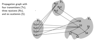
Propagation graphs are a mathematical modelling method for radio propagation channels. A propagation graph is a signal flow graph in which vertices represent transmitters, receivers or scatterers. Edges in the graph model propagation conditions between vertices. Propagation graph models were initially developed by Troels Pedersen, et al. for multipath propagation in scenarios with multiple scattering, such as indoor radio propagation. It has later been applied in many other scenarios.
This page is based on this Wikipedia article Text is available under the CC BY-SA 4.0 license; additional terms may apply. Images, videos and audio are available under their respective licenses.