This article may lack focus or may be about more than one topic. Please help improve this article, possibly by splitting the article and/or by introducing a disambiguation page, or discuss this issue on the talk page.(January 2024)
This article needs attention from an expert in Statistics. The specific problem is: It is unclear whether "statistical benchmarking" refers to one thing or several things.WikiProject Statistics may be able to help recruit an expert.(January 2024)
In statistics, benchmarking is a method of using auxiliary information to adjust the sampling weights used in an estimation process, in order to yield more accurate estimates of totals.
Suppose we have a population where each unit has a "value" associated with it. For example, could be a wage of an employee , or the cost of an item . Suppose we want to estimate the sum of all the . So we take a sample of the , get a sampling weight W(k) for all sampled , and then sum up for all sampled .
One property usually common to the weights described here is that if we sum them over all sampled , then this sum is an estimate of the total number of units in the population (for example, the total employment, or the total number of items). Because we have a sample, this estimate of the total number of units in the population will differ from the true population total. Similarly, the estimate of total (where we sum for all sampled ) will also differ from true population total.
We do not know what the true population total value is (if we did, there would be no point in sampling!). Yet often we do know what the sum of the are over all units in the population. For example, we may not know the total earnings of the population or the total cost of the population, but often we know the total employment or total volume of sales. And even if we don't know these exactly, there often are surveys done by other organizations or at earlier times, with very accurate estimates of these auxiliary quantities. One important function of a population census is to provide data that can be used for benchmarking smaller surveys.
The benchmarking procedure begins by first breaking the population into benchmarking cells. Cells are formed by grouping units together that share common characteristics, for example, similar , yet anything can be used that enhances the accuracy of the final estimates. For each cell , we let be the sum of all , where the sum is taken over all sampled in the cell . For each cell , we let be the auxiliary value for cell , which is commonly called the "benchmark target" for cell . Next, we compute a benchmark factor . Then, we adjust all weights by multiplying it by its benchmark factor , for its cell . The net result is that the estimated [formed by summing ] will now equal the benchmark target total . But the more important benefit is that the estimate of the total of [formed by summing ] will tend to be more accurate.
Relationship to stratified sampling
Benchmarking is sometimes referred to as 'post-stratification' because of its similarities to stratified sampling. The difference between the two is that in stratified sampling, we decide in advance how many units will be sampled from each stratum (equivalent to benchmarking cells); in benchmarking, we select units from the broader population, and the number chosen from each cell is a matter of chance.
The advantage of stratified sampling is that the sample numbers in each stratum can be controlled for desired accuracy outcomes. Without this control, we may end up with too much sample in one stratum and not enough in another – indeed, it's possible that a sample will contain no members from a certain cell, in which case benchmarking fails because , leading to a divide-by-zero problem. In such cases, it is necessary to 'collapse' cells together so that each remaining cell has an adequate sample size.
For this reason, benchmarking is generally used in situations where stratified sampling is impractical. For instance, when selecting people from a telephone directory, we can't tell what age they are so we can't easily stratify the sample by age. However, we can collect this information from the people sampled, allowing us to benchmark against demographic information.
Analysis of variance (ANOVA) is a collection of statistical models and their associated estimation procedures used to analyze the differences among means. ANOVA was developed by the statistician Ronald Fisher. ANOVA is based on the law of total variance, where the observed variance in a particular variable is partitioned into components attributable to different sources of variation. In its simplest form, ANOVA provides a statistical test of whether two or more population means are equal, and therefore generalizes the t-test beyond two means. In other words, the ANOVA is used to test the difference between two or more means.
Algorithms for calculating variance play a major role in computational statistics. A key difficulty in the design of good algorithms for this problem is that formulas for the variance may involve sums of squares, which can lead to numerical instability as well as to arithmetic overflow when dealing with large values.
In statistics, cluster sampling is a sampling plan used when mutually homogeneous yet internally heterogeneous groupings are evident in a statistical population. It is often used in marketing research.
In statistics, the standard deviation is a measure of the amount of variation of a random variable expected about its mean. A low standard deviation indicates that the values tend to be close to the mean of the set, while a high standard deviation indicates that the values are spread out over a wider range.
In statistics, stratified sampling is a method of sampling from a population which can be partitioned into subpopulations.
The weighted arithmetic mean is similar to an ordinary arithmetic mean, except that instead of each of the data points contributing equally to the final average, some data points contribute more than others. The notion of weighted mean plays a role in descriptive statistics and also occurs in a more general form in several other areas of mathematics.
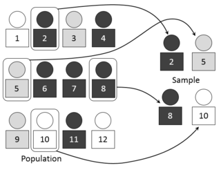
In statistics, quality assurance, and survey methodology, sampling is the selection of a subset or a statistical sample of individuals from within a statistical population to estimate characteristics of the whole population. Statisticians attempt to collect samples that are representative of the population. Sampling has lower costs and faster data collection compared to recording data from the entire population, and thus, it can provide insights in cases where it is infeasible to measure an entire population.
In statistics, the Pearson correlation coefficient (PCC) is a correlation coefficient that measures linear correlation between two sets of data. It is the ratio between the covariance of two variables and the product of their standard deviations; thus, it is essentially a normalized measurement of the covariance, such that the result always has a value between −1 and 1. As with covariance itself, the measure can only reflect a linear correlation of variables, and ignores many other types of relationships or correlations. As a simple example, one would expect the age and height of a sample of teenagers from a high school to have a Pearson correlation coefficient significantly greater than 0, but less than 1.
In statistics, the logistic model is a statistical model that models the log-odds of an event as a linear combination of one or more independent variables. In regression analysis, logistic regression is estimating the parameters of a logistic model. Formally, in binary logistic regression there is a single binary dependent variable, coded by an indicator variable, where the two values are labeled "0" and "1", while the independent variables can each be a binary variable or a continuous variable. The corresponding probability of the value labeled "1" can vary between 0 and 1, hence the labeling; the function that converts log-odds to probability is the logistic function, hence the name. The unit of measurement for the log-odds scale is called a logit, from logistic unit, hence the alternative names. See § Background and § Definition for formal mathematics, and § Example for a worked example.
Pearson's chi-squared test is a statistical test applied to sets of categorical data to evaluate how likely it is that any observed difference between the sets arose by chance. It is the most widely used of many chi-squared tests – statistical procedures whose results are evaluated by reference to the chi-squared distribution. Its properties were first investigated by Karl Pearson in 1900. In contexts where it is important to improve a distinction between the test statistic and its distribution, names similar to Pearson χ-squared test or statistic are used.
An F-test is any statistical test used to compare the variances of two samples or the ratio of variances between multiple samples. The test statistic, random variable F, is used to determine if the tested data has an F-distribution under the true null hypothesis, and true customary assumptions about the error term (ε). It is most often used when comparing statistical models that have been fitted to a data set, in order to identify the model that best fits the population from which the data were sampled. Exact "F-tests" mainly arise when the models have been fitted to the data using least squares. The name was coined by George W. Snedecor, in honour of Ronald Fisher. Fisher initially developed the statistic as the variance ratio in the 1920s.
Importance sampling is a Monte Carlo method for evaluating properties of a particular distribution, while only having samples generated from a different distribution than the distribution of interest. Its introduction in statistics is generally attributed to a paper by Teun Kloek and Herman K. van Dijk in 1978, but its precursors can be found in statistical physics as early as 1949. Importance sampling is also related to umbrella sampling in computational physics. Depending on the application, the term may refer to the process of sampling from this alternative distribution, the process of inference, or both.
In mathematics, Monte Carlo integration is a technique for numerical integration using random numbers. It is a particular Monte Carlo method that numerically computes a definite integral. While other algorithms usually evaluate the integrand at a regular grid, Monte Carlo randomly chooses points at which the integrand is evaluated. This method is particularly useful for higher-dimensional integrals.
Particle filters, or sequential Monte Carlo methods, are a set of Monte Carlo algorithms used to find approximate solutions for filtering problems for nonlinear state-space systems, such as signal processing and Bayesian statistical inference. The filtering problem consists of estimating the internal states in dynamical systems when partial observations are made and random perturbations are present in the sensors as well as in the dynamical system. The objective is to compute the posterior distributions of the states of a Markov process, given the noisy and partial observations. The term "particle filters" was first coined in 1996 by Pierre Del Moral about mean-field interacting particle methods used in fluid mechanics since the beginning of the 1960s. The term "Sequential Monte Carlo" was coined by Jun S. Liu and Rong Chen in 1998.
Sample size determination or estimation is the act of choosing the number of observations or replicates to include in a statistical sample. The sample size is an important feature of any empirical study in which the goal is to make inferences about a population from a sample. In practice, the sample size used in a study is usually determined based on the cost, time, or convenience of collecting the data, and the need for it to offer sufficient statistical power. In complex studies, different sample sizes may be allocated, such as in stratified surveys or experimental designs with multiple treatment groups. In a census, data is sought for an entire population, hence the intended sample size is equal to the population. In experimental design, where a study may be divided into different treatment groups, there may be different sample sizes for each group.
The goodness of fit of a statistical model describes how well it fits a set of observations. Measures of goodness of fit typically summarize the discrepancy between observed values and the values expected under the model in question. Such measures can be used in statistical hypothesis testing, e.g. to test for normality of residuals, to test whether two samples are drawn from identical distributions, or whether outcome frequencies follow a specified distribution. In the analysis of variance, one of the components into which the variance is partitioned may be a lack-of-fit sum of squares.
Bootstrapping is any test or metric that uses random sampling with replacement, and falls under the broader class of resampling methods. Bootstrapping assigns measures of accuracy to sample estimates. This technique allows estimation of the sampling distribution of almost any statistic using random sampling methods.
In statistics, the jackknife is a cross-validation technique and, therefore, a form of resampling. It is especially useful for bias and variance estimation. The jackknife pre-dates other common resampling methods such as the bootstrap. Given a sample of size , a jackknife estimator can be built by aggregating the parameter estimates from each subsample of size obtained by omitting one observation.
In survey methodology, the design effect is a measure of the expected impact of a sampling design on the variance of an estimator for some parameter. It is calculated as the ratio of the variance of an estimator based on a sample from an (often) complex sampling design, to the variance of an alternative estimator based on a simple random sample (SRS) of the same number of elements. The can be used to adjust the variance of an estimator in cases where the sample is not drawn using simple random sampling. It may also be useful in sample size calculations and for quantifying the representativeness of a sample. The term "design effect" was coined by Leslie Kish in 1965.
Inverse probability weighting is a statistical technique for estimating quantities related to a population other than the one from which the data was collected. Study designs with a disparate sampling population and population of target inference are common in application. There may be prohibitive factors barring researchers from directly sampling from the target population such as cost, time, or ethical concerns. A solution to this problem is to use an alternate design strategy, e.g. stratified sampling. Weighting, when correctly applied, can potentially improve the efficiency and reduce the bias of unweighted estimators.
This page is based on this Wikipedia article Text is available under the CC BY-SA 4.0 license; additional terms may apply. Images, videos and audio are available under their respective licenses.