Statistical stability

Last updated

The definition of statistical stability is the conclusion that the results or conclusion drawn from a statistical based testing are the dependence of the specific statistics on the sample size. To put simpler, the conclusion one draws from a survey or study is not only a dependent on the target sample, but on the surveyed group. If this size is large then the result is more stable, if smaller, then the conclusion is less stable. This effect is typical, for example, in relative frequencies (empirical probabilities) of mass events and averages. This phenomenon is widespread and so can be regarded as a fundamental natural phenomenon.

Contents

The physical nature of the statistical stability phenomenon is revealed by observing the mass events.

Currently, two theories are known that describe this phenomenon. The classical probability theory, which has a long history of development, and the theory of hyper-random phenomena, discovered in recent decades.

History

The first to draw attention to the phenomenon of statistical stability was the cloth merchant J. Graunt (1620–1674) [1] in 1662. Information about research on statistical stability is fragmentary for the period from the end of the seventeenth century to the end of the nineteenth century, e.g., by Jacob Bernoulli (1654–1705), Simeon Denis Poisson (1781–1840), Irenee-Jules Bienayme (1796–1878), Antoine Augustin Cournot (1801–1877), Adolphe Quetelet (1796–1874), John Venn (1834–1923), etc. [2] [3]

The systematic study of statistical stability began at the end of the nineteenth century. In 1879, the German statistician Wilhelm Lexis (1837–1914) made the first attempt to link the concept of statistical stability of the relative frequency with the dispersion. At the turn of the century and in the early twentieth century, statistical stability was studied by Karl Pearson (1857–1936), Alexander Alexandrovich Chuprov (1874–1926), Ladislaus Bortkiewicz (1868–1931), Andrey Markov (1856–1922), Richard von Mises (1883–1953), and others.

A new stage of experimental research began in the late twentieth century. Additional studies became necessary due to the new applied tasks and the detection of a number of phenomena that cannot be satisfactorily explained and described within the framework of the classical probability theory. The new tasks are, in particular, the ultra-precise measurement of physical quantities and ultra-precise forecasting of developments over large intervals of observation. The relatively new phenomena are, for instance, an unpredictable measurement progressive (drift) error, [4] [5] as well as a flicker noise, [6] which is detected everywhere and cannot be suppressed by averaging the data.

Statistical stability of the relative frequencies of events

Many well–known scientists led experimental investigations of the statistical stability phenomenon. It is known, for example, that coin-tossing experiments were studied by P.S. de Laplace (1749–1827), Georges-Louis Leclerc, Comte de Buffon (1707–1788), Karl Pearson, Nobel Prize Laureate Richard Feynman (1918–1988), Augustus de Morgan (1806–1871), William Stanley Jevons (1835–1882), Vsevolod Ivanovich Romanovsky (1879–1954), William Feller (1906–1970), and others. The trivial–at–first–glance task did not seem trivial for them. Table 1 presents some of the results of their experiments. [7] [8] [9] Table 2 shows the results described in [10] of ten runs of the same experiment in which each run consists of 1,000 tosses. The tables demonstrate that, for a large number of tosses, the relative frequency of heads or tails is close to 0.5.

Table 1. Results of coin-tossing experiments carried out by different scientists Table-1tif.tif
Table 1. Results of coin-tossing experiments carried out by different scientists
Table 2. Results of coin-tossing experiments described in the book (Mosteller et al. 1961) Table 2. Results of coin-tossing experiments described in the book (Mosteller et al. 1961).tiff
Table 2. Results of coin-tossing experiments described in the book (Mosteller et al. 1961)

Experimental studies of other real physical events show that for a high number of experiments the relative frequencies of events are stabilized; that shows the fundamental nature of the phenomenon of statistical stability.

Stability of statistics

The phenomenon of statistical stability is manifested not only in the stability of the relative frequency of mass events, but also in the stability of the average of the process, or its sample mean. The phenomenon of statistical stability is manifested in the case of averaging of fluctuations that are of different types, in particular, of the stochastic, determinate, and actual physical processes.

Example 1. In Fig. 1a and Fig. 1c the realization of noise with a uniform power spectral density (white noise) and a determinate period process are presented. In Fig. 1b and Fig. 1d the dependencies of the averages on the averaging interval are shown. As can be seen from Fig. 1b and Fig. 1d, when the averaging interval increases, fluctuations in the sample mean decrease and the average value gradually stabilizes.

Fig. 1. Realization of white Gaussian noise (a) and harmonic oscillation (c), together with the dependencies of the corresponding sample mean on the averaging interval (b, d) Fig. 1. Realization of white Gaussian noise (a) and harmonic oscillation (c), together with the dependencies of the corresponding sample mean on the average interval (b, d).tiff
Fig. 1. Realization of white Gaussian noise (a) and harmonic oscillation (c), together with the dependencies of the corresponding sample mean on the averaging interval (b, d)

Example 2. Fig. 2a and Fig. 2b show how the mains voltage in a city fluctuates quickly, while the average changes slowly. As the averaging interval increases from zero to one hour, the average voltage stabilizes (Fig. 2 b).

Fig. 2. Dependence of the mains voltage (a) and the corresponding average (b) on time over 1.8 hours Fig. 2. Dependence of the mains voltage (a) and the corresponding average (b) on time over 1.8 hours.tiff
Fig. 2. Dependence of the mains voltage (a) and the corresponding average (b) on time over 1.8 hours

The phenomenon of statistical stability is observed in the calculation also other statistics, in particular, sample moments.

Properties of statistical stability

Emergence

The statistical stability of the relative frequency is a property of mass (multiple) events. This property is not inherent in a single event, but is inherent in their collection. Similarly, the statistical stability of statistics is a property inherent to the set of samples. Therefore, the statistical stability of relative frequency or statistical stability of statistics can be regarded as an emergent property.

Hypothesis of perfect statistical stability

At first glance, it seems quite plausible that the sequence of relative frequencies of any real event should tend to a certain value (probability), and the sequence of the sample averages of discrete samples of any real process should have a limit , viz. , . This is the hypothesis of perfect (ideal) statistical stability. Probability theory is based on this hypothesis.[ dubious ]

Criticism of the hypothesis of perfect statistical stability

For many years, the hypothesis of ideal statistical stability was not in doubt, although some scholars (even Andrey Kolmogorov (1903–1987) [11] [12] [13] and such famous scientists as Andrey Markov, [14] Anatoliy Skorokhod (1930–2011), [15] Émile Borel (1871–1956), [16] V. N. Tutubalin [17] ), and others) noticed that, in the real world, this hypothesis is valid only with certain reservations.

The hypothesis of imperfect statistical stability

The possibility of adequate description of relative frequencies of actual events and sample averages of actual discrete samples by the expressions , is only a hypothesis. It does not follow from any experiments and any logical inferences. It is easy to demonstrate that not all processes, even oscillatory type, have the property of perfect statistical stability.

Example 3. In Fig. 3a and Fig. 3c two determinate oscillations are presented and in Fig. 3b and Fig. 3d are shown according to their averages. It is clear from Fig. 3b and Fig. 3d that in both cases, the average does not have a limit, i.e., both processes are statistically unstable.

Fig. 3. Statistically unstable oscillations (a, c) and corresponding averages (b, d) Fig. 3. Statistically unstable oscillations (a, c) and corresponding averages (b, d).tif
Fig. 3. Statistically unstable oscillations (a, c) and corresponding averages (b, d)

Experimental studies of various processes of different physical nature over broad observation intervals show that the hypothesis of perfect statistical stability is not confirmed'. The real world is continuously changing, and changes occur at all levels, including the statistical level. Statistical assessments formed on the basis of relatively small observation intervals are relatively stable. Their stability is manifested through a decrease in the fluctuation of statistical estimators when the volume of statistical data grows. This creates an illusion of perfect statistical stability. However, beyond a certain critical volume, the level of fluctuations remains practically unchanged (and sometimes even grows) when the amount of the data is increased. This indicates that the statistical stability is not perfect.

Example 4. Non-perfect statistical stability is illustrated Fig. 4 , [18] which presents mains voltage fluctuations over 2.5 days. Note the fluctuation in Fig. 2a shows beginning part of the fluctuation presented in Fig 4a. As can be seen from Fig. 4b, the sample average does not stabilize, even for very long averaging intervals.

Fig. 4. Dependence of the mains voltage (a) and the corresponding average (b) on time over 60 hours Fig. 4. Dependence of the mains voltage (a) and the corresponding average (b) on time over 60 hours.tif
Fig. 4. Dependence of the mains voltage (a) and the corresponding average (b) on time over 60 hours

Description of the phenomenon of statistical stability

Hilbert's sixth problem

Until the end of the nineteenth century probability theory was regarded as a physical discipline. At the Second International Congress of mathematicians (1900) David Hilbert (1862–1943) gave a speech entitled ‘Mathematical problems’. [19] Here he formulated what he considered to be the twenty three most important problems whose study could significantly stimulate the further development of science. The sixth problem was the mathematical description of the axioms of physics. In the part of his presentation relating to this problem, Hilbert noted that, in parallel with research on the foundations of geometry, one could approach the problem of an axiomatic construction, along the same lines, of the physical sciences in which mathematics played an exclusive role, and in particular, probability theory and mechanics.

Many scientists have responded to Hilbert's appeal. Among them were Richard von Mises, who considered the problem from the standpoint of natural science, and Andrey Kolmogorov, who proposed in 1929 the solution based on set theory and measure theory. The axiomatic approach proposed by A. N. Kolmogorov [20] is now favoured in probability theory. This approach has even been elevated to the rank of a standard. [21]

Description of the phenomenon of statistical stability in the framework of probability theory

Kolmogorov's probability theory is a typical mathematical discipline. In it, the subject matter is an abstract probability space and the scope of research is the mathematical relationships between its elements. The physical phenomenon of statistical stability of the relative frequency of events which constitutes the foundation of this discipline formally would not then appear to play any role. This phenomenon is taken into account in an idealized form by accepting the axiom of countable additivity, which is equivalent to acceptance of the hypothesis of perfect statistical stability.

Description of the phenomenon of statistical stability in the framework of the theory of hyper-random phenomena

In contrast to the classical mathematical probability theory, the theory of hyper-random phenomena is physical-mathematical one. Its subject matter is phenomenon of statistical stability and the scope of research is adequate description of it by so-called hyper-random models (hyper-random phenomena) taking into account the violation of statistical stability. [22]

The theory of hyper-random phenomena does not erase the achievements of probability theory and classical mathematical statistics, but complements them, extending the statements of these disciplines to a sphere in which they had not yet been considered where there is no convergence of statistics.

Parameters of statistical stability

There are a number of parameters characterizing the statistical stability, in particular, the parameters of statistical instability with respect to the average, the parameters of statistical instability with respect to the standard deviation, intervals of statistical stability with respect to the average, standard deviation, and other statistics, and so forth. The mathematically correct determination of these parameters and the development of a methodology for their estimation in case of unlimited and limited sample sizes are studied within the framework of the theory of hyper-random phenomena.

The areas of effective use of various approaches for description of the statistical stability phenomenon

The main parameters defining the bounds of the effective using of classical probability theory and the theory of hyper-random phenomena are intervals of statistical stability with respect to various statistics. Within these intervals the violations of statistical stability are negligible and therefore the use of probability theory is possible and reasonable. Outside these intervals the violations of statistical stability are essential and therefore it is necessary to use the methods that take into account these violations, in particular, the methods of the theory of hyper-random phenomena.

The limitations of statistical stability become apparent for large sample sizes and in the passage to the limit. Sample sizes are often small and therefore many practical tasks can be solved with acceptable accuracy using random (stochastic) models. Such models are usually simpler than the hyper-random models, so are preferred for not very large sample sizes. However, the hyper-random models have obvious advantages over the stochastic and other simpler models in cases when the limited statistical character of statistical stability becomes apparent, usually for long observation intervals and large sample sizes.

Therefore, the primary application of the hyper-random models is to statistically analyze various physical processes (electrical, magnetic, electromagnetic, acoustic, hydroacoustic, seismic-acoustic, meteorological, and others) of long duration, as well as high precision measurements of various physical quantities and the forecasting of physical processes by statistical processing of large data sets.

Twenty first century research shows that hyper-random models can be useful for solving other tasks too, for instance, in designing of radio electronic equipment. [23] [24]

See also

Related Research Articles

In statistics, an estimator is a rule for calculating an estimate of a given quantity based on observed data: thus the rule, the quantity of interest and its result are distinguished. For example, the sample mean is a commonly used estimator of the population mean.

<span class="mw-page-title-main">Frequentist probability</span> Interpretation of probability

Frequentist probability or frequentism is an interpretation of probability; it defines an event's probability as the limit of its relative frequency in many trials. Probabilities can be found by a repeatable objective process. The continued use of frequentist methods in scientific inference, however, has been called into question.

<span class="mw-page-title-main">Histogram</span> Graphical representation of the distribution of numerical data

A histogram is an approximate representation of the distribution of numerical data. The term was first introduced by Karl Pearson. To construct a histogram, the first step is to "bin" the range of values—that is, divide the entire range of values into a series of intervals—and then count how many values fall into each interval. The bins are usually specified as consecutive, non-overlapping intervals of a variable. The bins (intervals) must be adjacent and are often of equal size.

<span class="mw-page-title-main">Probability</span> Branch of mathematics concerning chance and uncertainty

Probability is the branch of mathematics concerning numerical descriptions of how likely an event is to occur, or how likely it is that a proposition is true. The probability of an event is a number between 0 and 1, where, roughly speaking, 0 indicates impossibility of the event and 1 indicates certainty. The higher the probability of an event, the more likely it is that the event will occur. A simple example is the tossing of a fair (unbiased) coin. Since the coin is fair, the two outcomes are both equally probable; the probability of "heads" equals the probability of "tails"; and since no other outcomes are possible, the probability of either "heads" or "tails" is 1/2.

The word probability has been used in a variety of ways since it was first applied to the mathematical study of games of chance. Does probability measure the real, physical, tendency of something to occur, or is it a measure of how strongly one believes it will occur, or does it draw on both these elements? In answering such questions, mathematicians interpret the probability values of probability theory.

Probability theory is the branch of mathematics concerned with probability. Although there are several different probability interpretations, probability theory treats the concept in a rigorous mathematical manner by expressing it through a set of axioms. Typically these axioms formalise probability in terms of a probability space, which assigns a measure taking values between 0 and 1, termed the probability measure, to a set of outcomes called the sample space. Any specified subset of the sample space is called an event. Central subjects in probability theory include discrete and continuous random variables, probability distributions, and stochastic processes . Although it is not possible to perfectly predict random events, much can be said about their behavior. Two major results in probability theory describing such behaviour are the law of large numbers and the central limit theorem.

<span class="mw-page-title-main">Probability distribution</span> Mathematical function for the probability a given outcome occurs in an experiment

In probability theory and statistics, a probability distribution is the mathematical function that gives the probabilities of occurrence of different possible outcomes for an experiment. It is a mathematical description of a random phenomenon in terms of its sample space and the probabilities of events.

<span class="mw-page-title-main">Statistical inference</span> Process of using data analysis

Statistical inference is the process of using data analysis to infer properties of an underlying distribution of probability. Inferential statistical analysis infers properties of a population, for example by testing hypotheses and deriving estimates. It is assumed that the observed data set is sampled from a larger population.

<span class="mw-page-title-main">Stochastic process</span> Collection of random variables

In probability theory and related fields, a stochastic or random process is a mathematical object usually defined as a family of random variables. Stochastic processes are widely used as mathematical models of systems and phenomena that appear to vary in a random manner. Examples include the growth of a bacterial population, an electrical current fluctuating due to thermal noise, or the movement of a gas molecule. Stochastic processes have applications in many disciplines such as biology, chemistry, ecology, neuroscience, physics, image processing, signal processing, control theory, information theory, computer science, cryptography and telecommunications. Furthermore, seemingly random changes in financial markets have motivated the extensive use of stochastic processes in finance.

<span class="mw-page-title-main">Law of large numbers</span> Averages of repeated trials converge to the expected value

In probability theory, the law of large numbers (LLN) is a theorem that describes the result of performing the same experiment a large number of times. According to the law, the average of the results obtained from a large number of trials should be close to the expected value and tends to become closer to the expected value as more trials are performed.

<span class="mw-page-title-main">Spectral density</span> Relative importance of certain frequencies in a composite signal

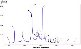
The power spectrum of a time series describes the distribution of power into frequency components composing that signal. According to Fourier analysis, any physical signal can be decomposed into a number of discrete frequencies, or a spectrum of frequencies over a continuous range. The statistical average of a certain signal or sort of signal as analyzed in terms of its frequency content, is called its spectrum.

<span class="mw-page-title-main">Confidence interval</span> Range of estimates for an unknown parameter

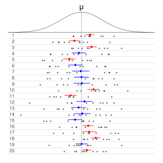
In frequentist statistics, a confidence interval (CI) is a range of estimates for an unknown parameter. A confidence interval is computed at a designated confidence level; the 95% confidence level is most common, but other levels, such as 90% or 99%, are sometimes used. The confidence level represents the long-run proportion of corresponding CIs that contain the true value of the parameter. For example, out of all intervals computed at the 95% level, 95% of them should contain the parameter's true value.

<span class="mw-page-title-main">Law of the iterated logarithm</span>

In probability theory, the law of the iterated logarithm describes the magnitude of the fluctuations of a random walk. The original statement of the law of the iterated logarithm is due to A. Ya. Khinchin (1924). Another statement was given by A. N. Kolmogorov in 1929.

This glossary of statistics and probability is a list of definitions of terms and concepts used in the mathematical sciences of statistics and probability, their sub-disciplines, and related fields. For additional related terms, see Glossary of mathematics and Glossary of experimental design.

In applied mathematics, the Wiener–Khinchin theorem or Wiener–Khintchine theorem, also known as the Wiener–Khinchin–Einstein theorem or the Khinchin–Kolmogorov theorem, states that the autocorrelation function of a wide-sense-stationary random process has a spectral decomposition given by the power spectrum of that process.

Intuitively, an algorithmically random sequence is a sequence of binary digits that appears random to any algorithm running on a universal Turing machine. The notion can be applied analogously to sequences on any finite alphabet. Random sequences are key objects of study in algorithmic information theory.

In statistics, the frequency of an event is the number of times the observation occurred/recorded in an experiment or study. These frequencies are often depicted graphically or in tabular form.

<span class="mw-page-title-main">Conditional probability</span> Probability of an event occurring, given that another event has already occurred

In probability theory, conditional probability is a measure of the probability of an event occurring, given that another event has already occurred. This particular method relies on event B occurring with some sort of relationship with another event A. In this event, the event B can be analyzed by a conditional probability with respect to A. If the event of interest is A and the event B is known or assumed to have occurred, "the conditional probability of A given B", or "the probability of A under the condition B", is usually written as P(A|B) or occasionally PB(A). This can also be understood as the fraction of probability B that intersects with A: .

References

  1. Graunt, J.: Natural and Political Observations Made Upon the Bills of Mortality. Baltimore (1939)
  2. Scheinin, O.B.: Teoriya Veroyatnostey. Istoricheskiy Ocherk (Probability Theory. Historical Review). http://www./ sheynin.de (2009). Accessed 21 June 2009
  3. Chaykovskiy, Yu.V.: O Prirode Sluchaynosti (About Random Nature). Centre for System Research, Institute of the History of Nature and Technique of the RAS, Moscow (2004)
  4. Sergeev, A.G., Krokhin, V.V.: Metrologiya (Metrology). Logos, Moscow (2001)
  5. Elyasberg, P.S.: Izmeritelnaya Informatsiya. Skolko ee Nuzhno? (Measuring Information. How Much Is Needed?). Nauka, Moscow (1983)
  6. Zhigalskiy, G.P.: Nonequilibrium γ noise in conducting films and contacts. Physics–Uspekhy. 46, 449–471 (2003)
  7. Gnedenko, B. V.: Kurs Teorii Veroyatnostey (Course on Probability Theory). Izdatelstvo physico–matematicheskoj literaturi, Moscow (1988)
  8. Feynman, R.P., Leighton, R.B., Sands M.: The Feynman Lectures on Physics. Vol. 1. Addison Wesley Publishing Company, Inc. Reading, Massachusetts–Palo Alto–London (1963)
  9. Rozhkov, V.A.: Teoriya Veroyatnostey Sluchainikh Sobytiy, Velichin i Funkziy s Gidrometeorologicheskimi Primerami (The Probability Theory of Random Events, Variables, and Functions with Hydrometeorological Examples). Progres–pogoda, Moscow (1996)
  10. Mosteller, F., Rourke, R.E.K., Thomas, G.B.: Probability: a First Course. Addison Wesley Publishing Company, Inc. Reading, Massachusetts–London (1961)
  11. Kolmogorov, A. N.: Teoriya veroyatnostey (Probability theory). In: Matematika, ee Metody i Znachenie (Mathematics, its Methods and Importance) 2, pp. 252–284 (1956)
  12. Kolmogorov, A. N. Osnovnye Ponyatiya Teorii Veroyatnostey (Fundamentals of Probability Theory). ONTI, Moscow (1974)
  13. Kolmogorov, A. N.: O logicheskikh osnovaniyakh teorii veroyatnostey (about logical foundations of probability theory). In: Teoriya veroyatnostey i matematicheskaya statistika (Probability theory and mathematical statistics), pp. 467–471. Nauka, Moscow (1986)
  14. Markov, A. A.: Ischislenie Veroyatnostey (Calculus of Probability). Moscow (1924)
  15. Ivanenko, V. I., Labkovsky, V. A.: Problema Neopredelennosty v Zadachakh Prinyatiya Resheniya (Uncertainty Problem in the Tasks of Decision Making). Naukova dumka, Kiev (1990)
  16. Borel, E.: Probabilité et Certitude. Presses Universitaires de France, Paris (1956)
  17. Tutubalin, V. N.: Teoriya Veroyatnostey (Probability Theory). Moskovskiy universitet, Moscow (1972)
  18. Gorban, I.I.: Phenomenon of statistical stability. Technical Physics 59(3), 333–340 (2014)
  19. Aleksandrov, P.S. (ed.): Problemy Hilberta (Hilbert's Problems). Nauka, Moscow (1969)
  20. Kolmogorov, A. N. Osnovnye Ponyatiya Teorii Veroyatnostey (Fundamentals of Probability Theory). ONTI, Moscow (1974)
  21. ISO 3534–1: Statistics. Vocabulary and symbols. Part I: General statistical terms and terms used in probability (2006)
  22. Gorban, I.I. The Statistical Stability Phenomenon – Springer, 2017. – 361 p. – ISBN   978-3-319-43584-8
  23. Uvarov, B.M.: Methods for representing the characteristics of radioelectronic equipment on the basis of the hyper-random phenomena theory. Radioelectronics and Communications Systems 53(10), 542–549 (2010)
  24. Zinkovskiy, Yu.F., Uvarov, B.M.: Hyper-randomness of algorithms for simulation of current radio electronic equipment. Radioelectronics and Communications Systems 54(3), 147–154 (2011)