In mathematics, the Dirac delta function is a generalized function or distribution introduced by the physicist Paul Dirac. It is used to model the density of an idealized point mass or point charge as a function equal to zero everywhere except for zero and whose integral over the entire real line is equal to one. As there is no function that has these properties, the computations made by the theoretical physicists appeared to mathematicians as nonsense until the introduction of distributions by Laurent Schwartz to formalize and validate the computations. As a distribution, the Dirac delta function is a linear functional that maps every function to its value at zero. The Kronecker delta function, which is usually defined on a discrete domain and takes values 0 and 1, is a discrete analog of the Dirac delta function.
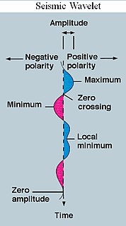
A wavelet is a wave-like oscillation with an amplitude that begins at zero, increases, and then decreases back to zero. It can typically be visualized as a "brief oscillation" like one recorded by a seismograph or heart monitor. Generally, wavelets are intentionally crafted to have specific properties that make them useful for signal processing. Using a "reverse, shift, multiply and integrate" technique called convolution, wavelets can be combined with known portions of a damaged signal to extract information from the unknown portions.

The Fourier transform (FT) decomposes a function of time into its constituent frequencies. This is similar to the way a musical chord can be expressed in terms of the volumes and frequencies of its constituent notes. The term Fourier transform refers to both the frequency domain representation and the mathematical operation that associates the frequency domain representation to a function of time. The Fourier transform of a function of time is itself a complex-valued function of frequency, whose magnitude component represents the amount of that frequency present in the original function, and whose complex argument is the phase offset of the basic sinusoid in that frequency. The Fourier transform is not limited to functions of time, but the domain of the original function is commonly referred to as the time domain. There is also an inverse Fourier transform that mathematically synthesizes the original function from its frequency domain representation.
In mathematics, the Fourier inversion theorem says that for many types of functions it is possible to recover a function from its Fourier transform. Intuitively it may be viewed as the statement that if we know all frequency and phase information about a wave then we may reconstruct the original wave precisely.

In mathematics, the Radon transform is the integral transform which takes a function f defined on the plane to a function Rf defined on the (two-dimensional) space of lines in the plane, whose value at a particular line is equal to the line integral of the function over that line. The transform was introduced in 1917 by Johann Radon, who also provided a formula for the inverse transform. Radon further included formulas for the transform in three dimensions, in which the integral is taken over planes. It was later generalized to higher-dimensional Euclidean spaces, and more broadly in the context of integral geometry. The complex analog of the Radon transform is known as the Penrose transform. The Radon transform is widely applicable to tomography, the creation of an image from the projection data associated with cross-sectional scans of an object.
In the theory of partial differential equations, elliptic operators are differential operators that generalize the Laplace operator. They are defined by the condition that the coefficients of the highest-order derivatives be positive, which implies the key property that the principal symbol is invertible, or equivalently that there are no real characteristic directions.
In mathematics, a Paley–Wiener theorem is any theorem that relates decay properties of a function or distribution at infinity with analyticity of its Fourier transform. The theorem is named for Raymond Paley (1907–1933) and Norbert Wiener (1894–1964). The original theorems did not use the language of distributions, and instead applied to square-integrable functions. The first such theorem using distributions was due to Laurent Schwartz.
In mathematics, the Hamilton–Jacobi equation (HJE) is a necessary condition describing extremal geometry in generalizations of problems from the calculus of variations, and is a special case of the Hamilton–Jacobi–Bellman equation. It is named for William Rowan Hamilton and Carl Gustav Jacob Jacobi.

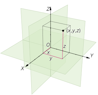
Oblate spheroidal coordinates are a three-dimensional orthogonal coordinate system that results from rotating the two-dimensional elliptic coordinate system about the non-focal axis of the ellipse, i.e., the symmetry axis that separates the foci. Thus, the two foci are transformed into a ring of radius in the x-y plane. Oblate spheroidal coordinates can also be considered as a limiting case of ellipsoidal coordinates in which the two largest semi-axes are equal in length.
Expected shortfall (ES) is a risk measure—a concept used in the field of financial risk measurement to evaluate the market risk or credit risk of a portfolio. The "expected shortfall at q% level" is the expected return on the portfolio in the worst % of cases. ES is an alternative to value at risk that is more sensitive to the shape of the tail of the loss distribution.
In mathematical analysis, Fourier integral operators have become an important tool in the theory of partial differential equations. The class of Fourier integral operators contains differential operators as well as classical integral operators as special cases.
In statistical signal processing, the goal of spectral density estimation (SDE) is to estimate the spectral density of a random signal from a sequence of time samples of the signal. Intuitively speaking, the spectral density characterizes the frequency content of the signal. One purpose of estimating the spectral density is to detect any periodicities in the data, by observing peaks at the frequencies corresponding to these periodicities.
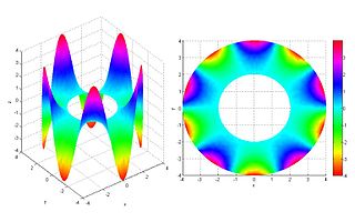
In mathematics, the Prolate spheroidal wave functions (PSWF) are a set of orthogonal badlimited functions. They are eigenfunctions of a timelimiting operation followed by a lowpassing operation. Let denote the time truncation operator, such that if and only if is timelimited within . Similarly, let denote an ideal low-pass filtering operator, such that if and only if is bandlimited within . The operator turns out to be linear, bounded and self-adjoint. For we denote with the n-th eigenfunction, defined as
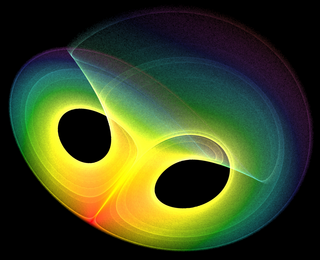
Bilinear time–frequency distributions, or quadratic time–frequency distributions, arise in a sub-field of signal analysis and signal processing called time–frequency signal processing, and, in the statistical analysis of time series data. Such methods are used where one needs to deal with a situation where the frequency composition of a signal may be changing over time; this sub-field used to be called time–frequency signal analysis, and is now more often called time–frequency signal processing due to the progress in using these methods to a wide range of signal-processing problems.
In mathematics, the FBI transform or Fourier–Bros–Iagolnitzer transform is a generalization of the Fourier transform developed by the French mathematical physicists Jacques Bros and Daniel Iagolnitzer in order to characterise the local analyticity of functions on Rn. The transform provides an alternative approach to analytic wave front sets of distributions, developed independently by the Japanese mathematicians Mikio Sato, Masaki Kashiwara and Takahiro Kawai in their approach to microlocal analysis. It can also be used to prove the analyticity of solutions of analytic elliptic partial differential equations as well as a version of the classical uniqueness theorem, strengthening the Cauchy–Kowalevski theorem, due to the Swedish mathematician Erik Albert Holmgren (1872–1943).
In mathematics, the Plancherel theorem for spherical functions is an important result in the representation theory of semisimple Lie groups, due in its final form to Harish-Chandra. It is a natural generalisation in non-commutative harmonic analysis of the Plancherel formula and Fourier inversion formula in the representation theory of the group of real numbers in classical harmonic analysis and has a similarly close interconnection with the theory of differential equations. It is the special case for zonal spherical functions of the general Plancherel theorem for semisimple Lie groups, also proved by Harish-Chandra. The Plancherel theorem gives the eigenfunction expansion of radial functions for the Laplacian operator on the associated symmetric space X; it also gives the direct integral decomposition into irreducible representations of the regular representation on L2(X). In the case of hyperbolic space, these expansions were known from prior results of Mehler, Weyl and Fock.
In the theory of partial differential equations, Holmgren's uniqueness theorem, or simply Holmgren's theorem, named after the Swedish mathematician Erik Albert Holmgren (1873–1943), is a uniqueness result for linear partial differential equations with real analytic coefficients.
Functional principal component analysis (FPCA) is a statistical method for investigating the dominant modes of variation of functional data. Using this method, a random function is represented in the eigenbasis, which is an orthonormal basis of the Hilbert space L2 that consists of the eigenfunctions of the autocovariance operator. FPCA represents functional data in the most parsimonious way, in the sense that when using a fixed number of basis functions, the eigenfunction basis explains more variation than any other basis expansion. FPCA can be applied for representing random functions, or in functional regression and classification.
The generalized functional linear model (GFLM) is an extension of the generalized linear model (GLM) that allows one to regress univariate responses of various types on functional predictors, which are mostly random trajectories generated by a square-integrable stochastic processes. Similarly to GLM, a link function relates the expected value of the response variable to a linear predictor, which in case of GFLM is obtained by forming the scalar product of the random predictor function with a smooth parameter function . Functional Linear Regression, Functional Poisson Regression and Functional Binomial Regression, with the important Functional Logistic Regression included, are special cases of GFLM. Applications of GFLM include classification and discrimination of stochastic processes and functional data.
Low-rank matrix approximations are essential tools in the application of kernel methods to large-scale learning problems.