In the mathematical field of differential geometry, the Riemann curvature tensor or Riemann–Christoffel tensor is the most common way used to express the curvature of Riemannian manifolds. It assigns a tensor to each point of a Riemannian manifold. It is a local invariant of Riemannian metrics which measures the failure of the second covariant derivatives to commute. A Riemannian manifold has zero curvature if and only if it is flat, i.e. locally isometric to the Euclidean space. The curvature tensor can also be defined for any pseudo-Riemannian manifold, or indeed any manifold equipped with an affine connection.
In the mathematical field of Riemannian geometry, the scalar curvature is a measure of the curvature of a Riemannian manifold. To each point on a Riemannian manifold, it assigns a single real number determined by the geometry of the metric near that point. It is defined by a complicated explicit formula in terms of partial derivatives of the metric components, although it is also characterized by the volume of infinitesimally small geodesic balls. In the context of the differential geometry of surfaces, the scalar curvature is twice the Gaussian curvature, and completely characterizes the curvature of a surface. In higher dimensions, however, the scalar curvature only represents one particular part of the Riemann curvature tensor.
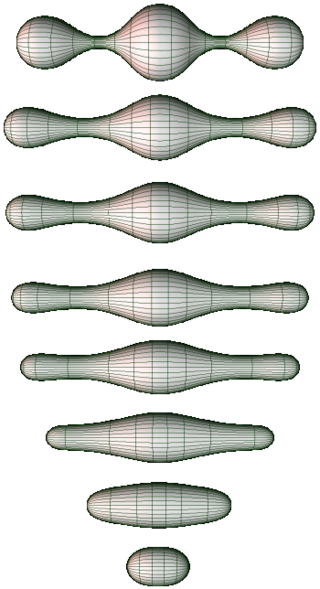
In the mathematical fields of differential geometry and geometric analysis, the Ricci flow, sometimes also referred to as Hamilton's Ricci flow, is a certain partial differential equation for a Riemannian metric. It is often said to be analogous to the diffusion of heat and the heat equation, due to formal similarities in the mathematical structure of the equation. However, it is nonlinear and exhibits many phenomena not present in the study of the heat equation.
In gauge theory and mathematical physics, a topological quantum field theory is a quantum field theory which computes topological invariants.
In mathematics, a Killing vector field, named after Wilhelm Killing, is a vector field on a Riemannian manifold that preserves the metric. Killing fields are the infinitesimal generators of isometries; that is, flows generated by Killing fields are continuous isometries of the manifold. More simply, the flow generates a symmetry, in the sense that moving each point of an object the same distance in the direction of the Killing vector will not distort distances on the object.
In quantum field theory, a nonlinear σ model describes a scalar field Σ which takes on values in a nonlinear manifold called the target manifold T. The non-linear σ-model was introduced by Gell-Mann & Lévy, who named it after a field corresponding to a spinless meson called σ in their model. This article deals primarily with the quantization of the non-linear sigma model; please refer to the base article on the sigma model for general definitions and classical (non-quantum) formulations and results.
When studying and formulating Albert Einstein's theory of general relativity, various mathematical structures and techniques are utilized. The main tools used in this geometrical theory of gravitation are tensor fields defined on a Lorentzian manifold representing spacetime. This article is a general description of the mathematics of general relativity.

Richard Melvin Schoen is an American mathematician known for his work in differential geometry and geometric analysis. He is best known for the resolution of the Yamabe problem in 1984.
In general relativity, the Gibbons–Hawking–York boundary term is a term that needs to be added to the Einstein–Hilbert action when the underlying spacetime manifold has a boundary.
The positive energy theorem refers to a collection of foundational results in general relativity and differential geometry. Its standard form, broadly speaking, asserts that the gravitational energy of an isolated system is nonnegative, and can only be zero when the system has no gravitating objects. Although these statements are often thought of as being primarily physical in nature, they can be formalized as mathematical theorems which can be proven using techniques of differential geometry, partial differential equations, and geometric measure theory.
In theoretical physics, a scalar–tensor theory is a field theory that includes both a scalar field and a tensor field to represent a certain interaction. For example, the Brans–Dicke theory of gravitation uses both a scalar field and a tensor field to mediate the gravitational interaction.
In mathematics, a metric connection is a connection in a vector bundle E equipped with a bundle metric; that is, a metric for which the inner product of any two vectors will remain the same when those vectors are parallel transported along any curve. This is equivalent to:
The Yamabe problem refers to a conjecture in the mathematical field of differential geometry, which was resolved in the 1980s. It is a statement about the scalar curvature of Riemannian manifolds:
Let (M,g) be a closed smooth Riemannian manifold. Then there exists a positive and smooth function f on M such that the Riemannian metric fg has constant scalar curvature.
In mathematics, and especially gauge theory, Seiberg–Witten invariants are invariants of compact smooth oriented 4-manifolds introduced by Edward Witten (1994), using the Seiberg–Witten theory studied by Nathan Seiberg and Witten during their investigations of Seiberg–Witten gauge theory.
The Hawking energy or Hawking mass is one of the possible definitions of mass in general relativity. It is a measure of the bending of ingoing and outgoing rays of light that are orthogonal to a 2-sphere surrounding the region of space whose mass is to be defined.
In Riemannian geometry, Schur's lemma is a result that says, heuristically, whenever certain curvatures are pointwise constant then they are forced to be globally constant. The proof is essentially a one-step calculation, which has only one input: the second Bianchi identity.
Lagrangian field theory is a formalism in classical field theory. It is the field-theoretic analogue of Lagrangian mechanics. Lagrangian mechanics is used to analyze the motion of a system of discrete particles each with a finite number of degrees of freedom. Lagrangian field theory applies to continua and fields, which have an infinite number of degrees of freedom.
In differential geometry, a complete Riemannian manifold is called a Ricci soliton if, and only if, there exists a smooth vector field such that
In mathematics, and especially differential geometry, the Quillen metric is a metric on the determinant line bundle of a family of operators. It was introduced by Daniel Quillen for certain elliptic operators over a Riemann surface, and generalized to higher-dimensional manifolds by Jean-Michel Bismut and Dan Freed.
In mathematics, and especially differential and algebraic geometry, K-stability is an algebro-geometric stability condition, for complex manifolds and complex algebraic varieties. The notion of K-stability was first introduced by Gang Tian and reformulated more algebraically later by Simon Donaldson. The definition was inspired by a comparison to geometric invariant theory (GIT) stability. In the special case of Fano varieties, K-stability precisely characterises the existence of Kähler–Einstein metrics. More generally, on any compact complex manifold, K-stability is conjectured to be equivalent to the existence of constant scalar curvature Kähler metrics.


