In evolutionary biology, fitness landscapes or adaptive landscapes (types of evolutionary landscapes) are used to visualize the relationship between genotypes and reproductive success. It is assumed that every genotype has a well-defined replication rate (often referred to as fitness). This fitness is the height of the landscape. Genotypes which are similar are said to be close to each other, while those that are very different are far from each other. The set of all possible genotypes, their degree of similarity, and their related fitness values is then called a fitness landscape. The idea of a fitness landscape is a metaphor to help explain flawed forms in evolution by natural selection, including exploits and glitches in animals like their reactions to supernormal stimuli.
The idea of studying evolution by visualizing the distribution of fitness values as a kind of landscape was first introduced by Sewall Wright in 1932.[1]
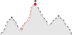
Sketch of a fitness landscape. The arrows indicate the preferred flow of a population on the landscape, and the points A and C are local optima. The red ball indicates a population that has moved from a very low fitness value to the top of a peak.
In all fitness landscapes, height represents and is a visual metaphor for fitness. There are three distinct ways of characterizing the other dimensions, though in each case distance represents and is a metaphor for degree of dissimilarity.[2]
Fitness landscapes are often conceived of as ranges of mountains. There exist local peaks (points from which all paths are downhill, i.e. to lower fitness) and valleys (regions from which many paths lead uphill). A fitness landscape with many local peaks surrounded by deep valleys is called rugged. If all genotypes have the same replication rate, on the other hand, a fitness landscape is said to be flat. An evolving population typically climbs uphill in the fitness landscape, by a series of small genetic changes, until – in the infinite time limit – a local optimum is reached.
Note that a local optimum cannot always be found even in evolutionary time: if the local optimum can be found in a reasonable amount of time then the fitness landscape is called "easy" and if the time required is exponential then the fitness landscape is called "hard".[3] Hard landscapes are characterized by the maze-like property by which an allele that was once beneficial becomes deleterious, forcing evolution to backtrack. However, the presence of the maze-like property in biophysically inspired fitness landscapes may not be sufficient to generate a hard landscape.[4]
Visualization of two dimensions of an NK fitness landscape. The arrows represent various mutational paths that the population could follow while evolving on the fitness landscape.
Genotype to fitness landscapes
Wright visualized a genotype space as a hypercube.[1] No continuous genotype "dimension" is defined. Instead, a network of genotypes are connected via mutational paths.
Stuart Kauffman's NK model falls into this category of fitness landscape. Newer network analysis techniques such as selection-weighted attraction graphing (SWAG) also use a dimensionless genotype space.[5]
Allele frequency to fitness landscapes
Wright's mathematical work described fitness as a function of allele frequencies.[2] Here, each dimension describes an allele frequency at a different gene, and goes between 0 and 1.
Phenotype to fitness landscapes
In the third kind of fitness landscape, each dimension represents a different phenotypic trait.[2] Under the assumptions of quantitative genetics, these phenotypic dimensions can be mapped onto genotypes. See the visualizations below for examples of phenotype to fitness landscapes.
Fitness seascapes extend the static fitness-landscape model by allowing the adaptive topography to shift through time or across changing environments. Rather than a fixed topography, seascapes describe adaptive surfaces whose peaks and valleys change in time as selection pressures evolve, producing trajectories that resemble dynamic "seascapes" rather than static landscapes which are necessary to accurately predict adaptation under time-varying selective conditions.[6][7]
Examples of factors that cause time-varying fitness landscapes are
Red Queen effects in which there is an interaction between two species which dynamically affects each one's fitness landscape.[9]
The concept has also been formalized in statistical-physical models that analyse time-dependent selection gradients, adaptive fluxes, and the movement of peaks in a changing environment. Fitness seascapes thus generalize traditional fitness landscapes by incorporating non-stationary selection, making them a useful framework for studying adaptation in fluctuating or clinically modulated environments.
In evolutionary optimization
Apart from the field of evolutionary biology, the concept of a fitness landscape has also gained importance in evolutionary optimization methods such as genetic algorithms or evolution strategies. In evolutionary optimization, one tries to solve real-world problems (e.g., engineering or logistics problems) by imitating the dynamics of biological evolution. For example, a delivery truck with a number of destination addresses can take a large variety of different routes, but only very few will result in a short driving time.
In order to use many common forms of evolutionary optimization, one has to define for every possible solutions to the problem of interest (i.e., every possible route in the case of the delivery truck) how 'good' it is. This is done by introducing a scalar-valued functionf(s) (scalar valued means that f(s) is a simple number, such as 0.3, while s can be a more complicated object, for example a list of destination addresses in the case of the delivery truck), which is called the fitness function.
A high f(s) implies that s is a good solution. In the case of the delivery truck, f(s) could be the number of deliveries per hour on route s. The best, or at least a very good, solution is then found in the following way: initially, a population of random solutions is created. Then, the solutions are mutated and selected for those with higher fitness, until a satisfying solution has been found.
Evolutionary optimization techniques are particularly useful in situations in which it is easy to determine the quality of a single solution, but hard to go through all possible solutions one by one (it is easy to determine the driving time for a particular route of the delivery truck, but it is almost impossible to check all possible routes once the number of destinations grows to more than a handful).
Even in cases where a fitness function is hard to define, the concept of a fitness landscape can be useful. For example, if fitness evaluation is by stochastic sampling, then sampling is from a (usually unknown) distribution at each point; nevertheless is can be useful to reason about the landscape formed by the expected fitness at each point. If fitness changes with time (dynamic optimisation) or with other species in the environment (co-evolution), it can still be useful to reason about the trajectories of the instantaneous fitness landscape. However, in some cases (for example, preference-based interactive evolutionary computation) the relevance is more limited, because there is no guarantee that human preferences are consistent with a single fitness assignment.
The concept of a scalar valued fitness function f(s) also corresponds to the concept of a potential or energy function in physics. The two concepts only differ in that physicists traditionally think in terms of minimizing the potential function, while biologists prefer the notion that fitness is being maximized. Therefore, taking the inverse of a potential function turns it into a fitness function, and vice versa.[10]
Caveats and limitations
Several important caveats exist. Since the human mind struggles to think in greater than three dimensions, 3D topologies can mislead when discussing highly multi-dimensional fitness landscapes.[11][12] In particular it is not clear whether peaks in natural biological fitness landscapes are ever truly separated by fitness valleys in such multidimensional landscapes, or whether they are connected by vastly long neutral ridges.[13][14] Additionally, the fitness landscape is not static in time but dependent on the changing environment and evolution of other genes.[5] It is hence more of a seascape,[15][16] further affecting how separated adaptive peaks can actually be. Additionally, it is relevant to take into account that a landscape is in general not an absolute but a relative function.[17] Finally, since it is common to use function as a proxy for fitness when discussing enzymes, any promiscuous activities exist as overlapping landscapes that together will determine the ultimate fitness of the organism, implying a gap between different coexisting relative landscapes.[18]
With these limitations in mind, fitness landscapes can still be an instructive way of thinking about evolution. It is fundamentally possible to measure (even if not to visualise) some of the parameters of landscape ruggedness and of peak number, height, separation, and clustering. Simplified 3D landscapes can then be used relative to each other to visually represent the relevant features. Additionally, fitness landscapes of small subsets of evolutionary pathways may be experimentally constructed and visualized, potentially revealing features such as fitness peaks and valleys.[5] Fitness landscapes of evolutionary pathways indicate the probable evolutionary steps and endpoints among sets of individual mutations.
↑ Mustonen, V; Lässig, M (2007). "From fitness landscapes to fitness seascapes: non-equilibrium dynamics of selection and adaptation". Trends in Genetics. 23 (10): 547–554. doi:10.1016/j.tig.2007.08.003.
↑ Mustonen, V; Lässig, M (2010). "Fitness flux and ubiquity of adaptive evolution". Proceedings of the National Academy of Sciences of the United States of America. 107 (24): 10165–10170. doi:10.1073/pnas.0907953107.
↑ Mustonen, Ville; Lässig, Michael (2009). "From fitness landscapes to seascapes: Non-equilibrium dynamics of selection and adaptation". Trends in Genetics. 25 (3): 111–9. doi:10.1016/j.tig.2009.01.002. PMID19232770.
↑ Mustonen, V; Lässig, M (2007). "From fitness landscapes to seascapes: non-equilibrium dynamics of selection and adaptation". Trends in Genetics. 23 (10): 547–554. doi:10.1016/j.tig.2007.08.003.
This page is based on this Wikipedia article Text is available under the CC BY-SA 4.0 license; additional terms may apply. Images, videos and audio are available under their respective licenses.