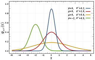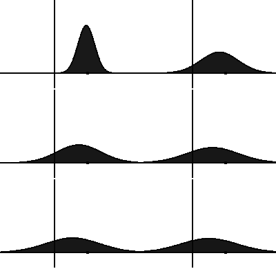
In probability theory and statistics, a normal distribution or Gaussian distribution is a type of continuous probability distribution for a real-valued random variable. The general form of its probability density function is The parameter is the mean or expectation of the distribution, while the parameter is the variance. The standard deviation of the distribution is (sigma). A random variable with a Gaussian distribution is said to be normally distributed, and is called a normal deviate.

In probability theory, the central limit theorem (CLT) states that, under appropriate conditions, the distribution of a normalized version of the sample mean converges to a standard normal distribution. This holds even if the original variables themselves are not normally distributed. There are several versions of the CLT, each applying in the context of different conditions.
The Black–Scholes or Black–Scholes–Merton model is a mathematical model for the dynamics of a financial market containing derivative investment instruments. From the parabolic partial differential equation in the model, known as the Black–Scholes equation, one can deduce the Black–Scholes formula, which gives a theoretical estimate of the price of European-style options and shows that the option has a unique price given the risk of the security and its expected return. The equation and model are named after economists Fischer Black and Myron Scholes. Robert C. Merton, who first wrote an academic paper on the subject, is sometimes also credited.

In statistical mechanics and information theory, the Fokker–Planck equation is a partial differential equation that describes the time evolution of the probability density function of the velocity of a particle under the influence of drag forces and random forces, as in Brownian motion. The equation can be generalized to other observables as well. The Fokker-Planck equation has multiple applications in information theory, graph theory, data science, finance, economics etc.
In mathematics, a Gaussian function, often simply referred to as a Gaussian, is a function of the base form and with parametric extension for arbitrary real constants a, b and non-zero c. It is named after the mathematician Carl Friedrich Gauss. The graph of a Gaussian is a characteristic symmetric "bell curve" shape. The parameter a is the height of the curve's peak, b is the position of the center of the peak, and c controls the width of the "bell".
In finance, the binomial options pricing model (BOPM) provides a generalizable numerical method for the valuation of options. Essentially, the model uses a "discrete-time" model of the varying price over time of the underlying financial instrument, addressing cases where the closed-form Black–Scholes formula is wanting.
In mathematical finance, the Greeks are the quantities representing the sensitivity of the price of a derivative instrument such as an option to changes in one or more underlying parameters on which the value of an instrument or portfolio of financial instruments is dependent. The name is used because the most common of these sensitivities are denoted by Greek letters. Collectively these have also been called the risk sensitivities, risk measures or hedge parameters.

A short-rate model, in the context of interest rate derivatives, is a mathematical model that describes the future evolution of interest rates by describing the future evolution of the short rate, usually written .
The relativistic Breit–Wigner distribution is a continuous probability distribution with the following probability density function,

The lattice Boltzmann methods (LBM), originated from the lattice gas automata (LGA) method (Hardy-Pomeau-Pazzis and Frisch-Hasslacher-Pomeau models), is a class of computational fluid dynamics (CFD) methods for fluid simulation. Instead of solving the Navier–Stokes equations directly, a fluid density on a lattice is simulated with streaming and collision (relaxation) processes. The method is versatile as the model fluid can straightforwardly be made to mimic common fluid behaviour like vapour/liquid coexistence, and so fluid systems such as liquid droplets can be simulated. Also, fluids in complex environments such as porous media can be straightforwardly simulated, whereas with complex boundaries other CFD methods can be hard to work with.

In mathematical finance, the Cox–Ingersoll–Ross (CIR) model describes the evolution of interest rates. It is a type of "one factor model" as it describes interest rate movements as driven by only one source of market risk. The model can be used in the valuation of interest rate derivatives. It was introduced in 1985 by John C. Cox, Jonathan E. Ingersoll and Stephen A. Ross as an extension of the Vasicek model, itself an Ornstein–Uhlenbeck process.
In finance, a volatility swap is a forward contract on the future realised volatility of a given underlying asset. Volatility swaps allow investors to trade the volatility of an asset directly, much as they would trade a price index. Its payoff at expiration is equal to
A local volatility model, in mathematical finance and financial engineering, is an option pricing model that treats volatility as a function of both the current asset level and of time . As such, it is a generalisation of the Black–Scholes model, where the volatility is a constant. Local volatility models are often compared with stochastic volatility models, where the instantaneous volatility is not just a function of the asset level but depends also on a new "global" randomness coming from an additional random component.

In mathematical finance, the Black–Scholes equation, also called the Black–Scholes–Merton equation, is a partial differential equation (PDE) governing the price evolution of derivatives under the Black–Scholes model. Broadly speaking, the term may refer to a similar PDE that can be derived for a variety of options, or more generally, derivatives.

In the theory of stochastic processes, a part of the mathematical theory of probability, the variance gamma (VG) process, also known as Laplace motion, is a Lévy process determined by a random time change. The process has finite moments, distinguishing it from many Lévy processes. There is no diffusion component in the VG process and it is thus a pure jump process. The increments are independent and follow a variance-gamma distribution, which is a generalization of the Laplace distribution.
The Press–Schechter formalism is a mathematical model for predicting the number of objects of a certain mass within a given volume of the Universe. It was described in an academic paper by William H. Press and Paul Schechter in 1974.
In quantum mechanics, and especially quantum information and the study of open quantum systems, the trace distanceT is a metric on the space of density matrices and gives a measure of the distinguishability between two states. It is the quantum generalization of the Kolmogorov distance for classical probability distributions.
In probability theory, the rectified Gaussian distribution is a modification of the Gaussian distribution when its negative elements are reset to 0. It is essentially a mixture of a discrete distribution and a continuous distribution as a result of censoring.
In mathematics and information theory, Sanov's theorem gives a bound on the probability of observing an atypical sequence of samples from a given probability distribution. In the language of large deviations theory, Sanov's theorem identifies the rate function for large deviations of the empirical measure of a sequence of i.i.d. random variables.
The redundancy principle in biology expresses the need of many copies of the same entity to fulfill a biological function. Examples are numerous: disproportionate numbers of spermatozoa during fertilization compared to one egg, large number of neurotransmitters released during neuronal communication compared to the number of receptors, large numbers of released calcium ions during transient in cells, and many more in molecular and cellular transduction or gene activation and cell signaling. This redundancy is particularly relevant when the sites of activation are physically separated from the initial position of the molecular messengers. The redundancy is often generated for the purpose of resolving the time constraint of fast-activating pathways. It can be expressed in terms of the theory of extreme statistics to determine its laws and quantify how the shortest paths are selected. The main goal is to estimate these large numbers from physical principles and mathematical derivations.


