
In special relativity, a four-vector is an object with four components, which transform in a specific way under Lorentz transformation. Specifically, a four-vector is an element of a four-dimensional vector space considered as a representation space of the standard representation of the Lorentz group, the (½,½) representation. It differs from a Euclidean vector in how its magnitude is determined. The transformations that preserve this magnitude are the Lorentz transformations, which include spatial rotations and boosts.
The primitive equations are a set of nonlinear differential equations that are used to approximate global atmospheric flow and are used in most atmospheric models. They consist of three main sets of balance equations:
- A continuity equation: Representing the conservation of mass.
- Conservation of momentum: Consisting of a form of the Navier–Stokes equations that describe hydrodynamical flow on the surface of a sphere under the assumption that vertical motion is much smaller than horizontal motion (hydrostasis) and that the fluid layer depth is small compared to the radius of the sphere
- A thermal energy equation: Relating the overall temperature of the system to heat sources and sinks

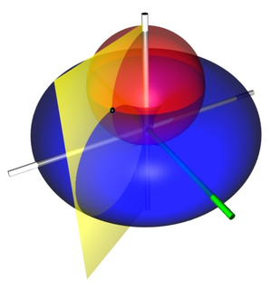
Parabolic coordinates are a two-dimensional orthogonal coordinate system in which the coordinate lines are confocal parabolas. A three-dimensional version of parabolic coordinates is obtained by rotating the two-dimensional system about the symmetry axis of the parabolas.
In physics, the Hamilton–Jacobi equation, named after William Rowan Hamilton and Carl Gustav Jacob Jacobi, is an alternative formulation of classical mechanics, equivalent to other formulations such as Newton's laws of motion, Lagrangian mechanics and Hamiltonian mechanics. The Hamilton–Jacobi equation is particularly useful in identifying conserved quantities for mechanical systems, which may be possible even when the mechanical problem itself cannot be solved completely.

Bipolar coordinates are a two-dimensional orthogonal coordinate system based on the Apollonian circles. Confusingly, the same term is also sometimes used for two-center bipolar coordinates. There is also a third system, based on two poles.

The Universal Transverse Mercator (UTM) is a system for assigning coordinates to locations on the surface of the Earth. Like the traditional method of latitude and longitude, it is a horizontal position representation, which means it ignores altitude and treats the earth as a perfect ellipsoid. However, it differs from global latitude/longitude in that it divides earth into 60 zones and projects each to the plane as a basis for its coordinates. Specifying a location means specifying the zone and the x, y coordinate in that plane. The projection from spheroid to a UTM zone is some parameterization of the transverse Mercator projection. The parameters vary by nation or region or mapping system.
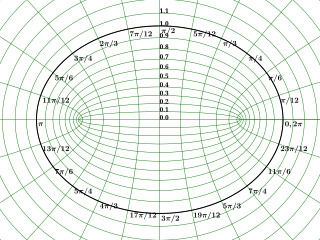
In geometry, the elliptic coordinate system is a two-dimensional orthogonal coordinate system in which the coordinate lines are confocal ellipses and hyperbolae. The two foci and are generally taken to be fixed at and , respectively, on the -axis of the Cartesian coordinate system.
Toroidal coordinates are a three-dimensional orthogonal coordinate system that results from rotating the two-dimensional bipolar coordinate system about the axis that separates its two foci. Thus, the two foci and in bipolar coordinates become a ring of radius in the plane of the toroidal coordinate system; the -axis is the axis of rotation. The focal ring is also known as the reference circle.
Bispherical coordinates are a three-dimensional orthogonal coordinate system that results from rotating the two-dimensional bipolar coordinate system about the axis that connects the two foci. Thus, the two foci and in bipolar coordinates remain points in the bispherical coordinate system.

Elliptic cylindrical coordinates are a three-dimensional orthogonal coordinate system that results from projecting the two-dimensional elliptic coordinate system in the perpendicular -direction. Hence, the coordinate surfaces are prisms of confocal ellipses and hyperbolae. The two foci and are generally taken to be fixed at and , respectively, on the -axis of the Cartesian coordinate system.

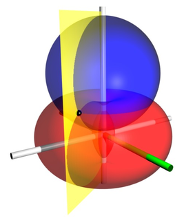
In mathematics, parabolic cylindrical coordinates are a three-dimensional orthogonal coordinate system that results from projecting the two-dimensional parabolic coordinate system in the perpendicular -direction. Hence, the coordinate surfaces are confocal parabolic cylinders. Parabolic cylindrical coordinates have found many applications, e.g., the potential theory of edges.

Prolate spheroidal coordinates are a three-dimensional orthogonal coordinate system that results from rotating the two-dimensional elliptic coordinate system about the focal axis of the ellipse, i.e., the symmetry axis on which the foci are located. Rotation about the other axis produces oblate spheroidal coordinates. Prolate spheroidal coordinates can also be considered as a limiting case of ellipsoidal coordinates in which the two smallest principal axes are equal in length.

Oblate spheroidal coordinates are a three-dimensional orthogonal coordinate system that results from rotating the two-dimensional elliptic coordinate system about the non-focal axis of the ellipse, i.e., the symmetry axis that separates the foci. Thus, the two foci are transformed into a ring of radius in the x-y plane. Oblate spheroidal coordinates can also be considered as a limiting case of ellipsoidal coordinates in which the two largest semi-axes are equal in length.
The intent of this article is to highlight the important points of the derivation of the Navier–Stokes equations as well as its application and formulation for different families of fluids.
The Cauchy momentum equation is a vector partial differential equation put forth by Cauchy that describes the non-relativistic momentum transport in any continuum.

In general relativity, a point mass deflects a light ray with impact parameter by an angle approximately equal to
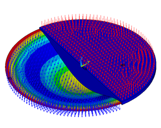
Bending of plates, or plate bending, refers to the deflection of a plate perpendicular to the plane of the plate under the action of external forces and moments. The amount of deflection can be determined by solving the differential equations of an appropriate plate theory. The stresses in the plate can be calculated from these deflections. Once the stresses are known, failure theories can be used to determine whether a plate will fail under a given load.
In the theory of Lorentzian manifolds, spherically symmetric spacetimes admit a family of nested round spheres. In such a spacetime, a particularly important kind of coordinate chart is the Schwarzschild chart, a kind of polar spherical coordinate chart on a static and spherically symmetric spacetime, which is adapted to these nested round spheres. The defining characteristic of Schwarzschild chart is that the radial coordinate possesses a natural geometric interpretation in terms of the surface area and Gaussian curvature of each sphere. However, radial distances and angles are not accurately represented.

In continuum mechanics, objective stress rates are time derivatives of stress that do not depend on the frame of reference. Many constitutive equations are designed in the form of a relation between a stress-rate and a strain-rate. The mechanical response of a material should not depend on the frame of reference. In other words, material constitutive equations should be frame-indifferent (objective). If the stress and strain measures are material quantities then objectivity is automatically satisfied. However, if the quantities are spatial, then the objectivity of the stress-rate is not guaranteed even if the strain-rate is objective.


