Oblate spheroidal coordinates

Last updated
Figure 1: Coordinate isosurfaces for a point P (shown as a black sphere) in oblate spheroidal coordinates (m, n, ph). The z-axis is vertical, and the foci are at +-2. The red oblate spheroid (flattened sphere) corresponds to m = 1, whereas the blue half-hyperboloid corresponds to n = 45deg. The azimuth ph = -60deg measures the dihedral angle between the green xz half-plane and the yellow half-plane that includes the point P. The Cartesian coordinates of P are roughly (1.09, -1.89, 1.66). Oblate spheroidal coordinates half hyperboloid.png
Figure 1: Coordinate isosurfaces for a point P (shown as a black sphere) in oblate spheroidal coordinates (μ, ν, φ). The z-axis is vertical, and the foci are at ±2. The red oblate spheroid (flattened sphere) corresponds to μ = 1, whereas the blue half-hyperboloid corresponds to ν = 45°. The azimuth φ = −60° measures the dihedral angle between the green xz half-plane and the yellow half-plane that includes the point P. The Cartesian coordinates of P are roughly (1.09, −1.89, 1.66).

Oblate spheroidal coordinates are a three-dimensional orthogonal coordinate system that results from rotating the two-dimensional elliptic coordinate system about the non-focal axis of the ellipse, i.e., the symmetry axis that separates the foci. Thus, the two foci are transformed into a ring of radius in the x-y plane. (Rotation about the other axis produces prolate spheroidal coordinates.) Oblate spheroidal coordinates can also be considered as a limiting case of ellipsoidal coordinates in which the two largest semi-axes are equal in length.

Contents

Oblate spheroidal coordinates are often useful in solving partial differential equations when the boundary conditions are defined on an oblate spheroid or a hyperboloid of revolution. For example, they played an important role in the calculation of the Perrin friction factors, which contributed to the awarding of the 1926 Nobel Prize in Physics to Jean Baptiste Perrin. These friction factors determine the rotational diffusion of molecules, which affects the feasibility of many techniques such as protein NMR and from which the hydrodynamic volume and shape of molecules can be inferred. Oblate spheroidal coordinates are also useful in problems of electromagnetism (e.g., dielectric constant of charged oblate molecules), acoustics (e.g., scattering of sound through a circular hole), fluid dynamics (e.g., the flow of water through a firehose nozzle) and the diffusion of materials and heat (e.g., cooling of a red-hot coin in a water bath)

Definition (μ,ν,φ)

Figure 2: Plot of the oblate spheroidal coordinates m and n in the x-z plane, where ph is zero and a equals one. The curves of constant m form red ellipses, whereas those of constant n form cyan half-hyperbolae in this plane. The z-axis runs vertically and separates the foci; the coordinates z and n always have the same sign. The surfaces of constant m and n in three dimensions are obtained by rotation about the z-axis, and are the red and blue surfaces, respectively, in Figure 1. OblateSpheroidCoord.png
Figure 2: Plot of the oblate spheroidal coordinates μ and ν in the x-z plane, where φ is zero and a equals one. The curves of constant μ form red ellipses, whereas those of constant ν form cyan half-hyperbolae in this plane. The z-axis runs vertically and separates the foci; the coordinates z and ν always have the same sign. The surfaces of constant μ and ν in three dimensions are obtained by rotation about the z-axis, and are the red and blue surfaces, respectively, in Figure 1.

The most common definition of oblate spheroidal coordinates is

where is a nonnegative real number and the angle . The azimuthal angle can fall anywhere on a full circle, between . These coordinates are favored over the alternatives below because they are not degenerate; the set of coordinates describes a unique point in Cartesian coordinates . The reverse is also true, except on the -axis and the disk in the -plane inside the focal ring.

Coordinate surfaces

The surfaces of constant μ form oblate spheroids, by the trigonometric identity

since they are ellipses rotated about the z-axis, which separates their foci. An ellipse in the x-z plane (Figure 2) has a major semiaxis of length a cosh μ along the x-axis, whereas its minor semiaxis has length a sinh μ along the z-axis. The foci of all the ellipses in the x-z plane are located on the x-axis at ±a.

Similarly, the surfaces of constant ν form one-sheet half hyperboloids of revolution by the hyperbolic trigonometric identity

For positive ν, the half-hyperboloid is above the x-y plane (i.e., has positive z) whereas for negative ν, the half-hyperboloid is below the x-y plane (i.e., has negative z). Geometrically, the angle ν corresponds to the angle of the asymptotes of the hyperbola. The foci of all the hyperbolae are likewise located on the x-axis at ±a.

Inverse transformation

The (μ, ν, φ) coordinates may be calculated from the Cartesian coordinates (x, y, z) as follows. The azimuthal angle φ is given by the formula

The cylindrical radius ρ of the point P is given by

and its distances to the foci in the plane defined by φ is given by

The remaining coordinates μ and ν can be calculated from the equations

where the sign of μ is always non-negative, and the sign of ν is the same as that of z.

Another method to compute the inverse transform is

where

Scale factors

The scale factors for the coordinates μ and ν are equal

whereas the azimuthal scale factor equals

Consequently, an infinitesimal volume element equals

and the Laplacian can be written

Other differential operators such as and can be expressed in the coordinates (μ, ν, φ) by substituting the scale factors into the general formulae found in orthogonal coordinates.

Basis Vectors

The orthonormal basis vectors for the coordinate system can be expressed in Cartesian coordinates as

where are the Cartesian unit vectors. Here, is the outward normal vector to the oblate spheroidal surface of constant , is the same azimuthal unit vector from spherical coordinates, and lies in the tangent plane to the oblate spheroid surface and completes the right-handed basis set.

Definition (ζ, ξ, φ)

Another set of oblate spheroidal coordinates are sometimes used where and (Smythe 1968). The curves of constant are oblate spheroids and the curves of constant are the hyperboloids of revolution. The coordinate is restricted by and is restricted by .

The relationship to Cartesian coordinates is

Scale factors

The scale factors for are:

Knowing the scale factors, various functions of the coordinates can be calculated by the general method outlined in the orthogonal coordinates article. The infinitesimal volume element is:

The gradient is:

The divergence is:

and the Laplacian equals

Oblate spheroidal harmonics

As is the case with spherical coordinates and spherical harmonics, Laplace's equation may be solved by the method of separation of variables to yield solutions in the form of oblate spheroidal harmonics, which are convenient to use when boundary conditions are defined on a surface with a constant oblate spheroidal coordinate.

Following the technique of separation of variables, a solution to Laplace's equation is written:

This yields three separate differential equations in each of the variables:

where m is a constant which is an integer because the φ variable is periodic with period 2π. n will then be an integer. The solution to these equations are:

where the are constants and and are associated Legendre polynomials of the first and second kind respectively. The product of the three solutions is called an oblate spheroidal harmonic and the general solution to Laplace's equation is written:

The constants will combine to yield only four independent constants for each harmonic.

Definition (σ, τ, φ)

Figure 3: Coordinate isosurfaces for a point P (shown as a black sphere) in the alternative oblate spheroidal coordinates (s, t, ph). As before, the oblate spheroid corresponding to s is shown in red, and ph measures the azimuthal angle between the green and yellow half-planes. However, the surface of constant t is a full one-sheet hyperboloid, shown in blue. This produces a two-fold degeneracy, shown by the two black spheres located at (x, y, +-z). Oblate spheroidal coordinates full hyperboloid.png
Figure 3: Coordinate isosurfaces for a point P (shown as a black sphere) in the alternative oblate spheroidal coordinates (σ, τ, φ). As before, the oblate spheroid corresponding to σ is shown in red, and φ measures the azimuthal angle between the green and yellow half-planes. However, the surface of constant τ is a full one-sheet hyperboloid, shown in blue. This produces a two-fold degeneracy, shown by the two black spheres located at (x, y, ±z).

An alternative and geometrically intuitive set of oblate spheroidal coordinates (σ, τ, φ) are sometimes used, where σ = cosh μ and τ = cos ν. [1] Therefore, the coordinate σ must be greater than or equal to one, whereas τ must lie between ±1, inclusive. The surfaces of constant σ are oblate spheroids, as were those of constant μ, whereas the curves of constant τ are full hyperboloids of revolution, including the half-hyperboloids corresponding to ±ν. Thus, these coordinates are degenerate; two points in Cartesian coordinates (x, y, ±z) map to one set of coordinates (σ, τ, φ). This two-fold degeneracy in the sign of z is evident from the equations transforming from oblate spheroidal coordinates to the Cartesian coordinates

The coordinates and have a simple relation to the distances to the focal ring. For any point, the sum of its distances to the focal ring equals , whereas their difference equals . Thus, the "far" distance to the focal ring is , whereas the "near" distance is .

Coordinate surfaces

Similar to its counterpart μ, the surfaces of constant σ form oblate spheroids

Similarly, the surfaces of constant τ form full one-sheet hyperboloids of revolution

Scale factors

The scale factors for the alternative oblate spheroidal coordinates are

whereas the azimuthal scale factor is .

Hence, the infinitesimal volume element can be written

and the Laplacian equals

Other differential operators such as and can be expressed in the coordinates by substituting the scale factors into the general formulae found in orthogonal coordinates.

As is the case with spherical coordinates, Laplaces equation may be solved by the method of separation of variables to yield solutions in the form of oblate spheroidal harmonics, which are convenient to use when boundary conditions are defined on a surface with a constant oblate spheroidal coordinate (See Smythe, 1968).

See also

Related Research Articles

<span class="mw-page-title-main">Lorentz transformation</span> Family of linear transformations

In physics, the Lorentz transformations are a six-parameter family of linear transformations from a coordinate frame in spacetime to another frame that moves at a constant velocity relative to the former. The respective inverse transformation is then parameterized by the negative of this velocity. The transformations are named after the Dutch physicist Hendrik Lorentz.

<span class="mw-page-title-main">Navier–Stokes equations</span> Equations describing the motion of viscous fluid substances

The Navier–Stokes equations are partial differential equations which describe the motion of viscous fluid substances. They were named after French engineer and physicist Claude-Louis Navier and the Irish physicist and mathematician George Gabriel Stokes. They were developed over several decades of progressively building the theories, from 1822 (Navier) to 1842–1850 (Stokes).

<span class="mw-page-title-main">Stress–energy tensor</span> Tensor describing energy momentum density in spacetime

The stress–energy tensor, sometimes called the stress–energy–momentum tensor or the energy–momentum tensor, is a tensor physical quantity that describes the density and flux of energy and momentum in spacetime, generalizing the stress tensor of Newtonian physics. It is an attribute of matter, radiation, and non-gravitational force fields. This density and flux of energy and momentum are the sources of the gravitational field in the Einstein field equations of general relativity, just as mass density is the source of such a field in Newtonian gravity.

In mathematical physics, n-dimensional de Sitter space is a maximally symmetric Lorentzian manifold with constant positive scalar curvature. It is the Lorentzian analogue of an n-sphere.

<span class="mw-page-title-main">Anti-de Sitter space</span> Maximally symmetric Lorentzian manifold with a negative cosmological constant

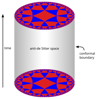
In mathematics and physics, n-dimensional anti-de Sitter space (AdSn) is a maximally symmetric Lorentzian manifold with constant negative scalar curvature. Anti-de Sitter space and de Sitter space are named after Willem de Sitter (1872–1934), professor of astronomy at Leiden University and director of the Leiden Observatory. Willem de Sitter and Albert Einstein worked together closely in Leiden in the 1920s on the spacetime structure of the universe. Paul Dirac was the first person to rigorously explore anti-de Sitter space, doing so in 1963.

In physics, the Hamilton–Jacobi equation, named after William Rowan Hamilton and Carl Gustav Jacob Jacobi, is an alternative formulation of classical mechanics, equivalent to other formulations such as Newton's laws of motion, Lagrangian mechanics and Hamiltonian mechanics.

In physics, the Polyakov action is an action of the two-dimensional conformal field theory describing the worldsheet of a string in string theory. It was introduced by Stanley Deser and Bruno Zumino and independently by L. Brink, P. Di Vecchia and P. S. Howe in 1976, and has become associated with Alexander Polyakov after he made use of it in quantizing the string in 1981. The action reads:

<span class="mw-page-title-main">Universal Transverse Mercator coordinate system</span> Map projection system

The Universal Transverse Mercator (UTM) is a map projection system for assigning coordinates to locations on the surface of the Earth. Like the traditional method of latitude and longitude, it is a horizontal position representation, which means it ignores altitude and treats the earth surface as a perfect ellipsoid. However, it differs from global latitude/longitude in that it divides earth into 60 zones and projects each to the plane as a basis for its coordinates. Specifying a location means specifying the zone and the x, y coordinate in that plane. The projection from spheroid to a UTM zone is some parameterization of the transverse Mercator projection. The parameters vary by nation or region or mapping system.

In the theory of general relativity, linearized gravity is the application of perturbation theory to the metric tensor that describes the geometry of spacetime. As a consequence, linearized gravity is an effective method for modeling the effects of gravity when the gravitational field is weak. The usage of linearized gravity is integral to the study of gravitational waves and weak-field gravitational lensing.

In physics and fluid mechanics, a Blasius boundary layer describes the steady two-dimensional laminar boundary layer that forms on a semi-infinite plate which is held parallel to a constant unidirectional flow. Falkner and Skan later generalized Blasius' solution to wedge flow, i.e. flows in which the plate is not parallel to the flow.

<span class="mw-page-title-main">Elliptic coordinate system</span> 2D coordinate system whose coordinate lines are confocal ellipses and hyperbolae

In geometry, the elliptic coordinate system is a two-dimensional orthogonal coordinate system in which the coordinate lines are confocal ellipses and hyperbolae. The two foci and are generally taken to be fixed at and , respectively, on the -axis of the Cartesian coordinate system.

<span class="mw-page-title-main">Toroidal coordinates</span>

Toroidal coordinates are a three-dimensional orthogonal coordinate system that results from rotating the two-dimensional bipolar coordinate system about the axis that separates its two foci. Thus, the two foci and in bipolar coordinates become a ring of radius in the plane of the toroidal coordinate system; the -axis is the axis of rotation. The focal ring is also known as the reference circle.

<span class="mw-page-title-main">Bispherical coordinates</span>

Bispherical coordinates are a three-dimensional orthogonal coordinate system that results from rotating the two-dimensional bipolar coordinate system about the axis that connects the two foci. Thus, the two foci and in bipolar coordinates remain points in the bispherical coordinate system.

<span class="mw-page-title-main">Bipolar cylindrical coordinates</span>

Bipolar cylindrical coordinates are a three-dimensional orthogonal coordinate system that results from projecting the two-dimensional bipolar coordinate system in the perpendicular -direction. The two lines of foci and of the projected Apollonian circles are generally taken to be defined by and , respectively, in the Cartesian coordinate system.

<span class="mw-page-title-main">Elliptic cylindrical coordinates</span>

Elliptic cylindrical coordinates are a three-dimensional orthogonal coordinate system that results from projecting the two-dimensional elliptic coordinate system in the perpendicular -direction. Hence, the coordinate surfaces are prisms of confocal ellipses and hyperbolae. The two foci and are generally taken to be fixed at and , respectively, on the -axis of the Cartesian coordinate system.

<span class="mw-page-title-main">Prolate spheroidal coordinates</span>

Prolate spheroidal coordinates are a three-dimensional orthogonal coordinate system that results from rotating the two-dimensional elliptic coordinate system about the focal axis of the ellipse, i.e., the symmetry axis on which the foci are located. Rotation about the other axis produces oblate spheroidal coordinates. Prolate spheroidal coordinates can also be considered as a limiting case of ellipsoidal coordinates in which the two smallest principal axes are equal in length.

Ellipsoidal coordinates are a three-dimensional orthogonal coordinate system that generalizes the two-dimensional elliptic coordinate system. Unlike most three-dimensional orthogonal coordinate systems that feature quadratic coordinate surfaces, the ellipsoidal coordinate system is based on confocal quadrics.

The Carter constant is a conserved quantity for motion around black holes in the general relativistic formulation of gravity. Its SI base units are kg2⋅m4⋅s−2. Carter's constant was derived for a spinning, charged black hole by Australian theoretical physicist Brandon Carter in 1968. Carter's constant along with the energy , axial angular momentum , and particle rest mass provide the four conserved quantities necessary to uniquely determine all orbits in the Kerr–Newman spacetime.

<span class="mw-page-title-main">Wrapped Cauchy distribution</span>

In probability theory and directional statistics, a wrapped Cauchy distribution is a wrapped probability distribution that results from the "wrapping" of the Cauchy distribution around the unit circle. The Cauchy distribution is sometimes known as a Lorentzian distribution, and the wrapped Cauchy distribution may sometimes be referred to as a wrapped Lorentzian distribution.

A proper reference frame in the theory of relativity is a particular form of accelerated reference frame, that is, a reference frame in which an accelerated observer can be considered as being at rest. It can describe phenomena in curved spacetime, as well as in "flat" Minkowski spacetime in which the spacetime curvature caused by the energy–momentum tensor can be disregarded. Since this article considers only flat spacetime—and uses the definition that special relativity is the theory of flat spacetime while general relativity is a theory of gravitation in terms of curved spacetime—it is consequently concerned with accelerated frames in special relativity.

References

  1. Abramowitz and Stegun, p. 752.

Bibliography

No angles convention

Angle convention

Unusual convention