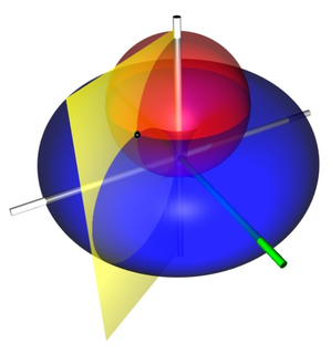
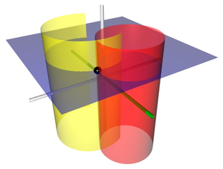
Last updated Coordinate surfaces of parabolic cylindrical coordinates. The red parabolic cylinder corresponds to σ=2, whereas the yellow parabolic cylinder corresponds to τ=1. The blue plane corresponds to z=2. These surfaces intersect at the point P (shown as a black sphere), which has Cartesian coordinates roughly (2, -1.5, 2).
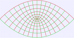
Parabolic coordinate system showing curves of constant σ and τ the horizontal and vertical axes are the x and y coordinates respectively. These coordinates are projected along the z-axis, and so this diagram will hold for any value of the z coordinate.
The parabolic cylindrical coordinates (σ, τ, z) are defined in terms of the Cartesian coordinates(x, y, z) by:
The surfaces of constant σ form confocal parabolic cylinders
that open towards +y, whereas the surfaces of constant τ form confocal parabolic cylinders
that open in the opposite direction, i.e., towards −y. The foci of all these parabolic cylinders are located along the line defined by x = y = 0. The radius r has a simple formula as well
Other differential operators can be expressed in the coordinates (σ, τ) by substituting the scale factors into the general formulae found in orthogonal coordinates.
Parabolic unit vectors expressed in terms of Cartesian unit vectors:
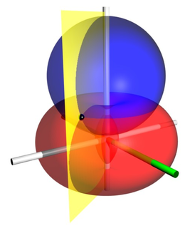
Parabolic cylinder harmonics
Since all of the surfaces of constant σ, τ and z are conicoids, Laplace's equation is separable in parabolic cylindrical coordinates. Using the technique of the separation of variables, a separated solution to Laplace's equation may be written:
and Laplace's equation, divided by V, is written:
Since the Z equation is separate from the rest, we may write
where m is constant. Z(z) has the solution:
Substituting −m2 for , Laplace's equation may now be written:
We may now separate the S and T functions and introduce another constant n2 to obtain:
The parabolic cylinder harmonics for (m, n) are now the product of the solutions. The combination will reduce the number of constants and the general solution to Laplace's equation may be written:
Korn GA, Korn TM (1961). Mathematical Handbook for Scientists and Engineers. New York: McGraw-Hill. p.181. LCCN59014456. ASIN B0000CKZX7.
Sauer R, Szabó I (1967). Mathematische Hilfsmittel des Ingenieurs. New York: Springer Verlag. p.96. LCCN67025285.
Zwillinger D (1992). Handbook of Integration. Boston, MA: Jones and Bartlett. p.114. ISBN0-86720-293-9. Same as Morse & Feshbach (1953), substituting uk for ξk.
Moon P, Spencer DE (1988). "Parabolic-Cylinder Coordinates (μ, ν, z)". Field Theory Handbook, Including Coordinate Systems, Differential Equations, and Their Solutions (corrected 2nd ed., 3rd printed.). New York: Springer-Verlag. pp.21–24 (Table 1.04). ISBN978-0-387-18430-2.
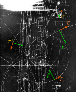
In physics the Lorentz force is the combination of electric and magnetic force on a point charge due to electromagnetic fields. A particle of charge q moving with a velocity v in an electric field E and a magnetic field B experiences a force of
In mathematics, a spherical coordinate system is a coordinate system for three-dimensional space where the position of a point is specified by three numbers: the radial distance of that point from a fixed origin, its polar angle measured from a fixed zenith direction, and the azimuthal angle of its orthogonal projection on a reference plane that passes through the origin and is orthogonal to the zenith, measured from a fixed reference direction on that plane. It can be seen as the three-dimensional version of the polar coordinate system.
In physics, the Navier–Stokes equations are certain partial differential equations which describe the motion of viscous fluid substances, named after French engineer and physicist Claude-Louis Navier and Anglo-Irish physicist and mathematician George Gabriel Stokes. They were developed over several decades of progressively building the theories, from 1822 (Navier) to 1842–1850 (Stokes).
In statistical mechanics, the Fokker–Planck equation is a partial differential equation that describes the time evolution of the probability density function of the velocity of a particle under the influence of drag forces and random forces, as in Brownian motion. The equation can be generalized to other observables as well.
Linear elasticity is a mathematical model of how solid objects deform and become internally stressed due to prescribed loading conditions. It is a simplification of the more general nonlinear theory of elasticity and a branch of continuum mechanics.
Parabolic coordinates are a two-dimensional orthogonal coordinate system in which the coordinate lines are confocal parabolas. A three-dimensional version of parabolic coordinates is obtained by rotating the two-dimensional system about the symmetry axis of the parabolas.
In physics, the Hamilton–Jacobi equation, named after William Rowan Hamilton and Carl Gustav Jacob Jacobi, is an alternative formulation of classical mechanics, equivalent to other formulations such as Newton's laws of motion, Lagrangian mechanics and Hamiltonian mechanics. The Hamilton–Jacobi equation is particularly useful in identifying conserved quantities for mechanical systems, which may be possible even when the mechanical problem itself cannot be solved completely.
Bipolar coordinates are a two-dimensional orthogonal coordinate system based on the Apollonian circles. Confusingly, the same term is also sometimes used for two-center bipolar coordinates. There is also a third system, based on two poles.
In continuum mechanics, the Cauchy stress tensor, true stress tensor, or simply called the stress tensor is a second order tensor named after Augustin-Louis Cauchy. The tensor consists of nine components that completely define the state of stress at a point inside a material in the deformed state, placement, or configuration. The tensor relates a unit-length direction vector n to the traction vector T(n) across an imaginary surface perpendicular to n:
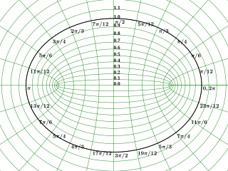
In geometry, the elliptic coordinate system is a two-dimensional orthogonal coordinate system in which the coordinate lines are confocal ellipses and hyperbolae. The two foci and are generally taken to be fixed at and , respectively, on the -axis of the Cartesian coordinate system.
Toroidal coordinates are a three-dimensional orthogonal coordinate system that results from rotating the two-dimensional bipolar coordinate system about the axis that separates its two foci. Thus, the two foci and in bipolar coordinates become a ring of radius in the plane of the toroidal coordinate system; the -axis is the axis of rotation. The focal ring is also known as the reference circle.
Bispherical coordinates are a three-dimensional orthogonal coordinate system that results from rotating the two-dimensional bipolar coordinate system about the axis that connects the two foci. Thus, the two foci and in bipolar coordinates remain points in the bispherical coordinate system.
Bipolar cylindrical coordinates are a three-dimensional orthogonal coordinate system that results from projecting the two-dimensional bipolar coordinate system in the perpendicular -direction. The two lines of foci and of the projected Apollonian circles are generally taken to be defined by and , respectively, in the Cartesian coordinate system.
Elliptic cylindrical coordinates are a three-dimensional orthogonal coordinate system that results from projecting the two-dimensional elliptic coordinate system in the perpendicular -direction. Hence, the coordinate surfaces are prisms of confocal ellipses and hyperbolae. The two foci and are generally taken to be fixed at and , respectively, on the -axis of the Cartesian coordinate system.
Prolate spheroidal coordinates are a three-dimensional orthogonal coordinate system that results from rotating the two-dimensional elliptic coordinate system about the focal axis of the ellipse, i.e., the symmetry axis on which the foci are located. Rotation about the other axis produces oblate spheroidal coordinates. Prolate spheroidal coordinates can also be considered as a limiting case of ellipsoidal coordinates in which the two smallest principal axes are equal in length.
Oblate spheroidal coordinates are a three-dimensional orthogonal coordinate system that results from rotating the two-dimensional elliptic coordinate system about the non-focal axis of the ellipse, i.e., the symmetry axis that separates the foci. Thus, the two foci are transformed into a ring of radius in the x-y plane. Oblate spheroidal coordinates can also be considered as a limiting case of ellipsoidal coordinates in which the two largest semi-axes are equal in length.
The intent of this article is to highlight the important points of the derivation of the Navier–Stokes equations as well as its application and formulation for different families of fluids.
In mathematics – specifically, in stochastic analysis – an Itô diffusion is a solution to a specific type of stochastic differential equation. That equation is similar to the Langevin equation used in physics to describe the Brownian motion of a particle subjected to a potential in a viscous fluid. Itô diffusions are named after the Japanese mathematician Kiyosi Itô.
The Cauchy momentum equation is a vector partial differential equation put forth by Cauchy that describes the non-relativistic momentum transport in any continuum.
In theoretical physics, relativistic Lagrangian mechanics is Lagrangian mechanics applied in the context of special relativity and general relativity.
This page is based on this Wikipedia article Text is available under the CC BY-SA 4.0 license; additional terms may apply. Images, videos and audio are available under their respective licenses.