Toroidal coordinates

Last updated
Illustration of toroidal coordinates, which are obtained by rotating a two-dimensional bipolar coordinate system about the axis separating its two foci. The foci are located at a distance 1 from the vertical z-axis. The portion of the red sphere that lies above the $xy$-plane is the s = 30deg isosurface, the blue torus is the t = 0.5 isosurface, and the yellow half-plane is the ph = 60deg isosurface. The green half-plane marks the x-z plane, from which ph is measured. The black point is located at the intersection of the red, blue and yellow isosurfaces, at Cartesian coordinates roughly (0.996, -1.725, 1.911). Toroidal coordinates.png
Illustration of toroidal coordinates, which are obtained by rotating a two-dimensional bipolar coordinate system about the axis separating its two foci. The foci are located at a distance 1 from the vertical z-axis. The portion of the red sphere that lies above the $xy$-plane is the σ = 30° isosurface, the blue torus is the τ = 0.5 isosurface, and the yellow half-plane is the φ = 60° isosurface. The green half-plane marks the x-z plane, from which φ is measured. The black point is located at the intersection of the red, blue and yellow isosurfaces, at Cartesian coordinates roughly (0.996, 1.725, 1.911).

Toroidal coordinates are a three-dimensional orthogonal coordinate system that results from rotating the two-dimensional bipolar coordinate system about the axis that separates its two foci. Thus, the two foci and in bipolar coordinates become a ring of radius in the plane of the toroidal coordinate system; the -axis is the axis of rotation. The focal ring is also known as the reference circle.

Contents

Definition

The most common definition of toroidal coordinates is

together with ). The coordinate of a point equals the angle and the coordinate equals the natural logarithm of the ratio of the distances and to opposite sides of the focal ring

The coordinate ranges are , and

Coordinate surfaces

Rotating this two-dimensional bipolar coordinate system about the vertical axis produces the three-dimensional toroidal coordinate system above. A circle on the vertical axis becomes the red sphere, whereas a circle on the horizontal axis becomes the blue torus. Apollonian circles.svg
Rotating this two-dimensional bipolar coordinate system about the vertical axis produces the three-dimensional toroidal coordinate system above. A circle on the vertical axis becomes the red sphere, whereas a circle on the horizontal axis becomes the blue torus.

Surfaces of constant correspond to spheres of different radii

that all pass through the focal ring but are not concentric. The surfaces of constant are non-intersecting tori of different radii

that surround the focal ring. The centers of the constant- spheres lie along the -axis, whereas the constant- tori are centered in the plane.

Inverse transformation

The coordinates may be calculated from the Cartesian coordinates (x, y, z) as follows. The azimuthal angle is given by the formula

The cylindrical radius of the point P is given by

and its distances to the foci in the plane defined by is given by

Geometric interpretation of the coordinates s and t of a point P. Observed in the plane of constant azimuthal angle
ph
{\displaystyle \phi }
, toroidal coordinates are equivalent to bipolar coordinates. The angle
s
{\displaystyle \sigma }
is formed by the two foci in this plane and P, whereas
t
{\displaystyle \tau }
is the logarithm of the ratio of distances to the foci. The corresponding circles of constant
s
{\displaystyle \sigma }
and
t
{\displaystyle \tau }
are shown in red and blue, respectively, and meet at right angles (magenta box); they are orthogonal. Bipolar coordinates.svg
Geometric interpretation of the coordinates σ and τ of a point P. Observed in the plane of constant azimuthal angle , toroidal coordinates are equivalent to bipolar coordinates. The angle is formed by the two foci in this plane and P, whereas is the logarithm of the ratio of distances to the foci. The corresponding circles of constant and are shown in red and blue, respectively, and meet at right angles (magenta box); they are orthogonal.

The coordinate equals the natural logarithm of the focal distances

whereas equals the angle between the rays to the foci, which may be determined from the law of cosines

Or explicitly, including the sign,

where .

The transformations between cylindrical and toroidal coordinates can be expressed in complex notation as

Scale factors

The scale factors for the toroidal coordinates and are equal

whereas the azimuthal scale factor equals

Thus, the infinitesimal volume element equals

Differential Operators

The Laplacian is given by

For a vector field

the Vector Laplacian is given by

Other differential operators such as and can be expressed in the coordinates by substituting the scale factors into the general formulae found in orthogonal coordinates.

Toroidal harmonics

Standard separation

The 3-variable Laplace equation

admits solution via separation of variables in toroidal coordinates. Making the substitution

A separable equation is then obtained. A particular solution obtained by separation of variables is:

where each function is a linear combination of:

Where P and Q are associated Legendre functions of the first and second kind. These Legendre functions are often referred to as toroidal harmonics.

Toroidal harmonics have many interesting properties. If you make a variable substitution then, for instance, with vanishing order (the convention is to not write the order when it vanishes) and

and

where and are the complete elliptic integrals of the first and second kind respectively. The rest of the toroidal harmonics can be obtained, for instance, in terms of the complete elliptic integrals, by using recurrence relations for associated Legendre functions.

The classic applications of toroidal coordinates are in solving partial differential equations, e.g., Laplace's equation for which toroidal coordinates allow a separation of variables or the Helmholtz equation, for which toroidal coordinates do not allow a separation of variables. Typical examples would be the electric potential and electric field of a conducting torus, or in the degenerate case, an electric current-ring (Hulme 1982).

An alternative separation

Alternatively, a different substitution may be made (Andrews 2006)

where

Again, a separable equation is obtained. A particular solution obtained by separation of variables is then:

where each function is a linear combination of:

Note that although the toroidal harmonics are used again for the T  function, the argument is rather than and the and indices are exchanged. This method is useful for situations in which the boundary conditions are independent of the spherical angle , such as the charged ring, an infinite half plane, or two parallel planes. For identities relating the toroidal harmonics with argument hyperbolic cosine with those of argument hyperbolic cotangent, see the Whipple formulae.

Related Research Articles

<span class="mw-page-title-main">Normal distribution</span> Probability distribution

In statistics, a normal distribution or Gaussian distribution is a type of continuous probability distribution for a real-valued random variable. The general form of its probability density function is

<span class="mw-page-title-main">Four-vector</span> 4-dimensional vector in relativity

In special relativity, a four-vector is an object with four components, which transform in a specific way under Lorentz transformations. Specifically, a four-vector is an element of a four-dimensional vector space considered as a representation space of the standard representation of the Lorentz group, the representation. It differs from a Euclidean vector in how its magnitude is determined. The transformations that preserve this magnitude are the Lorentz transformations, which include spatial rotations and boosts.

Linear elasticity is a mathematical model of how solid objects deform and become internally stressed due to prescribed loading conditions. It is a simplification of the more general nonlinear theory of elasticity and a branch of continuum mechanics.

In mathematical physics, n-dimensional de Sitter space is a maximally symmetric Lorentzian manifold with constant positive scalar curvature. It is the Lorentzian analogue of an n-sphere.

<span class="mw-page-title-main">Parabolic coordinates</span>

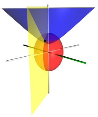
Parabolic coordinates are a two-dimensional orthogonal coordinate system in which the coordinate lines are confocal parabolas. A three-dimensional version of parabolic coordinates is obtained by rotating the two-dimensional system about the symmetry axis of the parabolas.

In physics, the Hamilton–Jacobi equation, named after William Rowan Hamilton and Carl Gustav Jacob Jacobi, is an alternative formulation of classical mechanics, equivalent to other formulations such as Newton's laws of motion, Lagrangian mechanics and Hamiltonian mechanics. The Hamilton–Jacobi equation is particularly useful in identifying conserved quantities for mechanical systems, which may be possible even when the mechanical problem itself cannot be solved completely.

In physics, the Polyakov action is an action of the two-dimensional conformal field theory describing the worldsheet of a string in string theory. It was introduced by Stanley Deser and Bruno Zumino and independently by L. Brink, P. Di Vecchia and P. S. Howe in 1976, and has become associated with Alexander Polyakov after he made use of it in quantizing the string in 1981. The action reads

<span class="mw-page-title-main">Bipolar coordinates</span> 2-dimensional orthogonal coordinate system based on Apollonian circles

Bipolar coordinates are a two-dimensional orthogonal coordinate system based on the Apollonian circles. Confusingly, the same term is also sometimes used for two-center bipolar coordinates. There is also a third system, based on two poles.

In probability and statistics, a circular distribution or polar distribution is a probability distribution of a random variable whose values are angles, usually taken to be in the range [0, 2π). A circular distribution is often a continuous probability distribution, and hence has a probability density, but such distributions can also be discrete, in which case they are called circular lattice distributions. Circular distributions can be used even when the variables concerned are not explicitly angles: the main consideration is that there is not usually any real distinction between events occurring at the lower or upper end of the range, and the division of the range could notionally be made at any point.

<span class="mw-page-title-main">Elliptic coordinate system</span> 2D coordinate system whose coordinate lines are confocal ellipses and hyperbolae

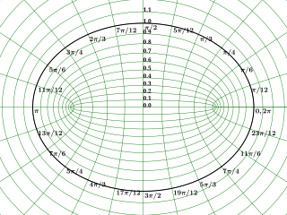
In geometry, the elliptic coordinate system is a two-dimensional orthogonal coordinate system in which the coordinate lines are confocal ellipses and hyperbolae. The two foci and are generally taken to be fixed at and , respectively, on the -axis of the Cartesian coordinate system.

<span class="mw-page-title-main">Bispherical coordinates</span>

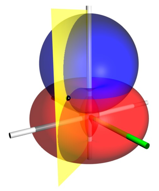
Bispherical coordinates are a three-dimensional orthogonal coordinate system that results from rotating the two-dimensional bipolar coordinate system about the axis that connects the two foci. Thus, the two foci and in bipolar coordinates remain points in the bispherical coordinate system.

<span class="mw-page-title-main">Bipolar cylindrical coordinates</span>

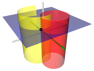
Bipolar cylindrical coordinates are a three-dimensional orthogonal coordinate system that results from projecting the two-dimensional bipolar coordinate system in the perpendicular -direction. The two lines of foci and Failed to parse : F_{2} of the projected Apollonian circles are generally taken to be defined by and , respectively, in the Cartesian coordinate system.

<span class="mw-page-title-main">Elliptic cylindrical coordinates</span>

Elliptic cylindrical coordinates are a three-dimensional orthogonal coordinate system that results from projecting the two-dimensional elliptic coordinate system in the perpendicular -direction. Hence, the coordinate surfaces are prisms of confocal ellipses and hyperbolae. The two foci and are generally taken to be fixed at and , respectively, on the -axis of the Cartesian coordinate system.

<span class="mw-page-title-main">Prolate spheroidal coordinates</span>

Prolate spheroidal coordinates are a three-dimensional orthogonal coordinate system that results from rotating the two-dimensional elliptic coordinate system about the focal axis of the ellipse, i.e., the symmetry axis on which the foci are located. Rotation about the other axis produces oblate spheroidal coordinates. Prolate spheroidal coordinates can also be considered as a limiting case of ellipsoidal coordinates in which the two smallest principal axes are equal in length.

<span class="mw-page-title-main">Oblate spheroidal coordinates</span> Three-dimensional orthogonal coordinate system

Oblate spheroidal coordinates are a three-dimensional orthogonal coordinate system that results from rotating the two-dimensional elliptic coordinate system about the non-focal axis of the ellipse, i.e., the symmetry axis that separates the foci. Thus, the two foci are transformed into a ring of radius in the x-y plane. Oblate spheroidal coordinates can also be considered as a limiting case of ellipsoidal coordinates in which the two largest semi-axes are equal in length.

Ellipsoidal coordinates are a three-dimensional orthogonal coordinate system that generalizes the two-dimensional elliptic coordinate system. Unlike most three-dimensional orthogonal coordinate systems that feature quadratic coordinate surfaces, the ellipsoidal coordinate system is based on confocal quadrics.

In the theory of special functions, Whipple's transformation for Legendre functions, named after Francis John Welsh Whipple, arise from a general expression, concerning associated Legendre functions. These formulae have been presented previously in terms of a viewpoint aimed at spherical harmonics, now that we view the equations in terms of toroidal coordinates, whole new symmetries of Legendre functions arise.

In physics and mathematics, the κ-Poincaré group, named after Henri Poincaré, is a quantum group, obtained by deformation of the Poincaré group into a Hopf algebra. It is generated by the elements and with the usual constraint:

<span class="mw-page-title-main">Bending of plates</span>

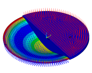
Bending of plates, or plate bending, refers to the deflection of a plate perpendicular to the plane of the plate under the action of external forces and moments. The amount of deflection can be determined by solving the differential equations of an appropriate plate theory. The stresses in the plate can be calculated from these deflections. Once the stresses are known, failure theories can be used to determine whether a plate will fail under a given load.

In theoretical physics, more specifically in quantum field theory and supersymmetry, supersymmetric Yang–Mills, also known as super Yang–Mills and abbreviated to SYM, is a supersymmetric generalization of Yang–Mills theory, which is a gauge theory that plays an important part in the mathematical formulation of forces in particle physics.

References

Bibliography