Circulation (physics)

Last updated October 26, 2023

In physics, circulation is the line integral of a vector field around a closed curve. In fluid dynamics, the field is the fluid velocity field. In electrodynamics, it can be the electric or the magnetic field.

Definition and properties

If $V$ is a vector field and $d l$ is a vector representing the differential length of a small element of a defined curve, the contribution of that differential length to circulation is $dΓ$ :

\mathrm {d} \Gamma =\mathbf {V} \cdot \mathrm {d} \mathbf {l} =\left|\mathbf {V} \right|\left|\mathrm {d} \mathbf {l} \right|\cos \theta .

Here, $θ$ is the angle between the vectors $V$ and $d l$ .

The circulation $Γ$ of a vector field $V$ around a closed curve $C$ is the line integral:^[1]^[2]

\Gamma =\oint _{C}\mathbf {V} \cdot \mathrm {d} \mathbf {l} .

In a conservative vector field this integral evaluates to zero for every closed curve. That means that a line integral between any two points in the field is independent of the path taken. It also implies that the vector field can be expressed as the gradient of a scalar function, which is called a potential.^[2]

Relation to vorticity and curl

Circulation can be related to curl of a vector field $V$ and, more specifically, to vorticity if the field is a fluid velocity field,

{\boldsymbol {\omega }}=\nabla \times \mathbf {V} .

By Stokes' theorem, the flux of curl or vorticity vectors through a surface S is equal to the circulation around its perimeter,^[2]

\Gamma =\oint _{\partial S}\mathbf {V} \cdot \mathrm {d} \mathbf {l} =\iint _{S}\nabla \times \mathbf {V} \cdot \mathrm {d} \mathbf {S} =\iint _{S}{\boldsymbol {\omega }}\cdot \mathrm {d} \mathbf {S}

Here, the closed integration path $\partialS$ is the boundary or perimeter of an open surface $S$ , whose infinitesimal element normal $d S = n dS$ is oriented according to the right-hand rule. Thus curl and vorticity are the circulation per unit area, taken around a local infinitesimal loop.

In potential flow of a fluid with a region of vorticity, all closed curves that enclose the vorticity have the same value for circulation.^[3]

Uses

Kutta–Joukowski theorem in fluid dynamics

In fluid dynamics, the lift per unit span (L') acting on a body in a two-dimensional flow field is directly proportional to the circulation, i.e. it can be expressed as the product of the circulation Γ about the body, the fluid density $\rho _{\infty }$ , and the speed of the body relative to the free-stream $v_{\infty }$ :

L'=\rho _{\infty }v_{\infty }\Gamma

This is known as the Kutta–Joukowski theorem.^[4]

This equation applies around airfoils, where the circulation is generated by airfoil action; and around spinning objects experiencing the Magnus effect where the circulation is induced mechanically. In airfoil action, the magnitude of the circulation is determined by the Kutta condition.^[4]

The circulation on every closed curve around the airfoil has the same value, and is related to the lift generated by each unit length of span. Provided the closed curve encloses the airfoil, the choice of curve is arbitrary.^[3]

Circulation is often used in computational fluid dynamics as an intermediate variable to calculate forces on an airfoil or other body.

Fundamental equations of electromagnetism

In electrodynamics, the Maxwell-Faraday law of induction can be stated in two equivalent forms:^[5] that the curl of the electric field is equal to the negative rate of change of the magnetic field,

\nabla \times \mathbf {E} =-{\frac {\partial \mathbf {B} }{\partial t}}

or that the circulation of the electric field around a loop is equal to the negative rate of change of the magnetic field flux through any surface spanned by the loop, by Stokes' theorem

\oint _{\partial S}\mathbf {E} \cdot \mathrm {d} \mathbf {l} =\iint _{S}\nabla \times \mathbf {E} \cdot \mathrm {d} \mathbf {S} =-{\frac {\mathrm {d} }{\mathrm {d} t}}\int _{S}\mathbf {B} \cdot \mathrm {d} \mathbf {S} .

Circulation of a static magnetic field is, by Ampère's law, proportional to the total current enclosed by the loop

\oint _{\partial S}\mathbf {B} \cdot \mathrm {d} \mathbf {l} =\mu _{0}\iint _{S}\mathbf {J} \cdot \mathrm {d} \mathbf {S} =\mu _{0}I_{\text{enc}}.

For systems with electric fields that change over time, the law must be modified to include a term known as Maxwell's correction.

Related Research Articles

In vector calculus, the curl, also known as rotor, is a vector operator that describes the infinitesimal circulation of a vector field in three-dimensional Euclidean space. The curl at a point in the field is represented by a vector whose length and direction denote the magnitude and axis of the maximum circulation. The curl of a field is formally defined as the circulation density at each point of the field.

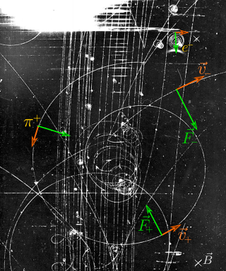
In physics, the Lorentz force is the combination of electric and magnetic force on a point charge due to electromagnetic fields. A particle of charge $q$ moving with a velocity $v$ in an electric field $E$ and a magnetic field $B$ experiences a force of

Maxwell's equations, or Maxwell–Heaviside equations, are a set of coupled partial differential equations that, together with the Lorentz force law, form the foundation of classical electromagnetism, classical optics, and electric circuits. The equations provide a mathematical model for electric, optical, and radio technologies, such as power generation, electric motors, wireless communication, lenses, radar, etc. They describe how electric and magnetic fields are generated by charges, currents, and changes of the fields. The equations are named after the physicist and mathematician James Clerk Maxwell, who, in 1861 and 1862, published an early form of the equations that included the Lorentz force law. Maxwell first used the equations to propose that light is an electromagnetic phenomenon. The modern form of the equations in their most common formulation is credited to Oliver Heaviside.

In vector calculus and differential geometry the generalized Stokes theorem, also called the Stokes–Cartan theorem, is a statement about the integration of differential forms on manifolds, which both simplifies and generalizes several theorems from vector calculus. In particular, the fundamental theorem of calculus is the special case where the manifold is a line segment, Green’s theorem and Stokes' theorem are the cases of a surface in $or and the divergence theorem is the case of a volume in Hence, the theorem is sometimes referred to as the Fundamental Theorem of Multivariate Calculus .$

Flux describes any effect that appears to pass or travel through a surface or substance. Flux is a concept in applied mathematics and vector calculus which has many applications to physics. For transport phenomena, flux is a vector quantity, describing the magnitude and direction of the flow of a substance or property. In vector calculus flux is a scalar quantity, defined as the surface integral of the perpendicular component of a vector field over a surface.

<span class="mw-page-title-main">Vector field</span> Assignment of a vector to each point in a subset of Euclidean space

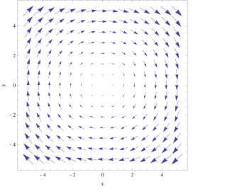
In vector calculus and physics, a vector field is an assignment of a vector to each point in a space, most commonly Euclidean space $. A vector field on a plane can be visualized as a collection of arrows with given magnitudes and directions, each attached to a point on the plane. Vector fields are often used to model, for example, the speed and direction of a moving fluid throughout three dimensional space, such as the wind, or the strength and direction of some force, such as the magnetic or gravitational force, as it changes from one point to another point.$

In vector calculus, the divergence theorem, also known as Gauss's theorem or Ostrogradsky's theorem, is a theorem which relates the flux of a vector field through a closed surface to the divergence of the field in the volume enclosed.

In classical electromagnetism, Ampère's circuital law relates the circulation of a magnetic field around a closed loop to the electric current passing through the loop.

In vector calculus, Green's theorem relates a line integral around a simple closed curve $C$ to a double integral over the plane region $D$ bounded by $C$ . It is the two-dimensional special case of Stokes' theorem.

In vector calculus, a conservative vector field is a vector field that is the gradient of some function. A conservative vector field has the property that its line integral is path independent; the choice of any path between two points does not change the value of the line integral. Path independence of the line integral is equivalent to the vector field under the line integral being conservative. A conservative vector field is also irrotational; in three dimensions, this means that it has vanishing curl. An irrotational vector field is necessarily conservative provided that the domain is simply connected.

<span class="mw-page-title-main">Scalar potential</span> When potential energy difference depends only on displacement

In mathematical physics, scalar potential, simply stated, describes the situation where the difference in the potential energies of an object in two different positions depends only on the positions, not upon the path taken by the object in traveling from one position to the other. It is a scalar field in three-space: a directionless value (scalar) that depends only on its location. A familiar example is potential energy due to gravity.

In electromagnetism, displacement current density is the quantity $\partial D /\partial t$ appearing in Maxwell's equations that is defined in terms of the rate of change of $D$ , the electric displacement field. Displacement current density has the same units as electric current density, and it is a source of the magnetic field just as actual current is. However it is not an electric current of moving charges, but a time-varying electric field. In physical materials, there is also a contribution from the slight motion of charges bound in atoms, called dielectric polarization.

In physics and mathematics, in the area of vector calculus, Helmholtz's theorem, also known as the fundamental theorem of vector calculus, states that any sufficiently smooth, rapidly decaying vector field in three dimensions can be resolved into the sum of an irrotational (curl-free) vector field and a solenoidal (divergence-free) vector field; this is known as the Helmholtz decomposition or Helmholtz representation. It is named after Hermann von Helmholtz.

The gradient theorem, also known as the fundamental theorem of calculus for line integrals, says that a line integral through a gradient field can be evaluated by evaluating the original scalar field at the endpoints of the curve. The theorem is a generalization of the second fundamental theorem of calculus to any curve in a plane or space rather than just the real line.

In fluid mechanics, Kelvin's circulation theorem states:

In a barotropic, ideal fluid with conservative body forces, the circulation around a closed curve moving with the fluid remains constant with time.

In physics, a quantum vortex represents a quantized flux circulation of some physical quantity. In most cases, quantum vortices are a type of topological defect exhibited in superfluids and superconductors. The existence of quantum vortices was first predicted by Lars Onsager in 1949 in connection with superfluid helium. Onsager reasoned that quantisation of vorticity is a direct consequence of the existence of a superfluid order parameter as a spatially continuous wavefunction. Onsager also pointed out that quantum vortices describe the circulation of superfluid and conjectured that their excitations are responsible for superfluid phase transitions. These ideas of Onsager were further developed by Richard Feynman in 1955 and in 1957 were applied to describe the magnetic phase diagram of type-II superconductors by Alexei Alexeyevich Abrikosov. In 1935 Fritz London published a very closely related work on magnetic flux quantization in superconductors. London's fluxoid can also be viewed as a quantum vortex.

The Kutta–Joukowski theorem is a fundamental theorem in aerodynamics used for the calculation of lift of an airfoil translating in a uniform fluid at a constant speed large enough so that the flow seen in the body-fixed frame is steady and unseparated. The theorem relates the lift generated by an airfoil to the speed of the airfoil through the fluid, the density of the fluid and the circulation around the airfoil. The circulation is defined as the line integral around a closed loop enclosing the airfoil of the component of the velocity of the fluid tangent to the loop. It is named after Martin Kutta and Nikolai Zhukovsky who first developed its key ideas in the early 20th century. Kutta–Joukowski theorem is an inviscid theory, but it is a good approximation for real viscous flow in typical aerodynamic applications.

In mathematics, a line integral is an integral where the function to be integrated is evaluated along a curve. The terms path integral, curve integral, and curvilinear integral are also used; contour integral is used as well, although that is typically reserved for line integrals in the complex plane.

Stokes' theorem, also known as the Kelvin–Stokes theorem after Lord Kelvin and George Stokes, the fundamental theorem for curls or simply the curl theorem, is a theorem in vector calculus on $. Given a vector field, the theorem relates the integral of the curl of the vector field over some surface, to the line integral of the vector field around the boundary of the surface. The classical theorem of Stokes can be stated in one sentence: The line integral of a vector field over a loop is equal to the flux of its curl through the enclosed surface. It is illustrated in the figure, where the direction of positive circulation of the bounding contour \partialΣ, and the direction n of positive flux through the surface Σ, are related by a right-hand-rule. For the right hand the fingers circulate along \partialΣ and the thumb is directed along n .$

In fluid dynamics, Prandtl–Batchelor theorem states that if in a two-dimensional laminar flow at high Reynolds number closed streamlines occur, then the vorticity in the closed streamline region must be a constant. A similar statement holds true for axisymmetric flows. The theorem is named after Ludwig Prandtl and George Batchelor. Prandtl in his celebrated 1904 paper stated this theorem in arguments, George Batchelor unaware of this work proved the theorem in 1956. The problem was also studied in the same year by Richard Feynman and Paco Lagerstrom and by W.W. Wood in 1957.

References

↑ Robert W. Fox; Alan T. McDonald; Philip J. Pritchard (2003). Introduction to Fluid Mechanics (6 ed.). Wiley. ISBN 978-0-471-20231-8.
1 2 3 "The Feynman Lectures on Physics Vol. II Ch. 3: Vector Integral Calculus". feynmanlectures.caltech.edu. Retrieved 2020-11-02.
1 2 Anderson, John D. (1984), Fundamentals of Aerodynamics, section 3.16. McGraw-Hill. ISBN 0-07-001656-9
1 2 A.M. Kuethe; J.D. Schetzer (1959). Foundations of Aerodynamics (2 ed.). John Wiley & Sons. §4.11. ISBN 978-0-471-50952-3.
↑ "The Feynman Lectures on Physics Vol. II Ch. 17: The Laws of Induction". feynmanlectures.caltech.edu. Retrieved 2020-11-02.

This page is based on this Wikipedia article
Text is available under the CC BY-SA 4.0 license; additional terms may apply.
Images, videos and audio are available under their respective licenses.

[1] Robert W. Fox; Alan T. McDonald; Philip J. Pritchard (2003). Introduction to Fluid Mechanics (6 ed.). Wiley. ISBN 978-0-471-20231-8.

[:0-2] 1 2 3 "The Feynman Lectures on Physics Vol. II Ch. 3: Vector Integral Calculus". feynmanlectures.caltech.edu. Retrieved 2020-11-02.

[JDA-3] 1 2 Anderson, John D. (1984), Fundamentals of Aerodynamics, section 3.16. McGraw-Hill. ISBN 0-07-001656-9

[K&S-4] 1 2 A.M. Kuethe; J.D. Schetzer (1959). Foundations of Aerodynamics (2 ed.). John Wiley & Sons. §4.11. ISBN 978-0-471-50952-3.

[5] "The Feynman Lectures on Physics Vol. II Ch. 17: The Laws of Induction". feynmanlectures.caltech.edu. Retrieved 2020-11-02.

[1]

[2]

[3]

[4]

[5]