Faraday's law of induction

Last updated

Faraday's experiment showing induction between coils of wire: The liquid battery (right) provides a current which flows through the small coil (A), creating a magnetic field. When the coils are stationary, no current is induced. But when the small coil is moved in or out of the large coil (B), the magnetic flux through the large coil changes, inducing a current which is detected by the galvanometer (G). Induction experiment.png
Faraday's experiment showing induction between coils of wire: The liquid battery (right) provides a current which flows through the small coil (A), creating a magnetic field. When the coils are stationary, no current is induced. But when the small coil is moved in or out of the large coil (B), the magnetic flux through the large coil changes, inducing a current which is detected by the galvanometer (G).

Faraday's law of induction (or simply Faraday's law) is a law of electromagnetism predicting how a magnetic field will interact with an electric circuit to produce an electromotive force (emf). This phenomenon, known as electromagnetic induction, is the fundamental operating principle of transformers, inductors, and many types of electric motors, generators and solenoids. [2] [3]

Contents

The Maxwell–Faraday equation (listed as one of Maxwell's equations) describes the fact that a spatially varying (and also possibly time-varying, depending on how a magnetic field varies in time) electric field always accompanies a time-varying magnetic field, while Faraday's law states that there is emf (electromotive force, defined as electromagnetic work done on a unit charge when it has traveled one round of a conductive loop) on a conductive loop when the magnetic flux through the surface enclosed by the loop varies in time.

Faraday's law had been discovered and one aspect of it (transformer emf) was formulated as the Maxwell–Faraday equation later. The equation of Faraday's law can be derived by the Maxwell–Faraday equation (describing transformer emf) and the Lorentz force (describing motional emf). The integral form of the Maxwell–Faraday equation describes only the transformer emf, while the equation of Faraday's law describes both the transformer emf and the motional emf.

History

Electromagnetic induction was discovered independently by Michael Faraday in 1831 and Joseph Henry in 1832. [4] Faraday was the first to publish the results of his experiments. [5] [6]

Faraday's 1831 demonstration Faraday emf experiment.svg
Faraday's 1831 demonstration

Faraday's notebook on August 29, 1831 [8] describes an experimental demonstration of electromagnetic induction (see figure) [9] that wraps two wires around opposite sides of an iron ring (like a modern toroidal transformer). His assessment of newly-discovered properties of electromagnets suggested that when current started to flow in one wire, a sort of wave would travel through the ring and cause some electrical effect on the opposite side. Indeed, a galvanometer's needle measured a transient current (which he called a "wave of electricity") on the right side's wire when he connected or disconnected the left side's wire to a battery. [10] :182–183 This induction was due to the change in magnetic flux that occurred when the battery was connected and disconnected. [7] His notebook entry also noted that fewer wraps for the battery side resulted in a greater disturbance of the galvanometer's needle. [8]

Within two months, Faraday had found several other manifestations of electromagnetic induction. For example, he saw transient currents when he quickly slid a bar magnet in and out of a coil of wires, and he generated a steady (DC) current by rotating a copper disk near the bar magnet with a sliding electrical lead ("Faraday's disk"). [10] :191–195

Faraday's disk, the first electric generator, a type of homopolar generator Faraday disk generator.jpg
Faraday's disk, the first electric generator, a type of homopolar generator

Michael Faraday explained electromagnetic induction using a concept he called lines of force. However, scientists at the time widely rejected his theoretical ideas, mainly because they were not formulated mathematically. [10] :510 An exception was James Clerk Maxwell, who in 1861–62 used Faraday's ideas as the basis of his quantitative electromagnetic theory. [10] :510 [11] [12] In Maxwell's papers, the time-varying aspect of electromagnetic induction is expressed as a differential equation which Oliver Heaviside referred to as Faraday's law even though it is different from the original version of Faraday's law, and does not describe motional emf. Heaviside's version (see Maxwell–Faraday equation below) is the form recognized today in the group of equations known as Maxwell's equations.

Lenz's law, formulated by Emil Lenz in 1834, [13] describes "flux through the circuit", and gives the direction of the induced emf and current resulting from electromagnetic induction (elaborated upon in the examples below).

According to Albert Einstein, much of the groundwork and discovery of his special relativity theory was presented by this law of induction by Faraday in 1834. [14] [15]

Faraday's law

Alternating electric current flows through the solenoid on the left, producing a changing magnetic field. This field causes, by electromagnetic induction, an electric current to flow in the wire loop on the right. Electromagnetic induction - solenoid to loop - animation.gif
Alternating electric current flows through the solenoid on the left, producing a changing magnetic field. This field causes, by electromagnetic induction, an electric current to flow in the wire loop on the right.

The most widespread version of Faraday's law states:

The electromotive force around a closed path is equal to the negative of the time rate of change of the magnetic flux enclosed by the path. [16] [17]

Mathematical statement

The definition of surface integral relies on splitting the surface S into small surface elements. Each element is associated with a vector dA of magnitude equal to the area of the element and with direction normal to the element and pointing "outward" (with respect to the orientation of the surface). Surface integral illustration.svg
The definition of surface integral relies on splitting the surface Σ into small surface elements. Each element is associated with a vector dA of magnitude equal to the area of the element and with direction normal to the element and pointing "outward" (with respect to the orientation of the surface).

For a loop of wire in a magnetic field, the magnetic flux ΦB is defined for any surface Σ whose boundary is the given loop. Since the wire loop may be moving, we write Σ(t) for the surface. The magnetic flux is the surface integral:

where dA is an element of area vector of the moving surface Σ(t), B is the magnetic field, and B · dA is a vector dot product representing the element of flux through dA. In more visual terms, the magnetic flux through the wire loop is proportional to the number of magnetic field lines that pass through the loop.

When the flux changes—because B changes, or because the wire loop is moved or deformed, or both—Faraday's law of induction says that the wire loop acquires an emf, defined as the energy available from a unit charge that has traveled once around the wire loop. [18] :ch17 [19] [20] (Although some sources state the definition differently, this expression was chosen for compatibility with the equations of special relativity.) Equivalently, it is the voltage that would be measured by cutting the wire to create an open circuit, and attaching a voltmeter to the leads.

Faraday's law states that the emf is also given by the rate of change of the magnetic flux:

where is the electromotive force (emf) and ΦB is the magnetic flux.

The direction of the electromotive force is given by Lenz's law.

The laws of induction of electric currents in mathematical form was established by Franz Ernst Neumann in 1845. [21]

Faraday's law contains the information about the relationships between both the magnitudes and the directions of its variables. However, the relationships between the directions are not explicit; they are hidden in the mathematical formula.

A Left Hand Rule for Faraday's Law. The sign of DPhB, the change in flux, is found based on the relationship between the magnetic field B, the area of the loop A, and the normal n to that area, as represented by the fingers of the left hand. If DPhB is positive, the direction of the emf is the same as that of the curved fingers (yellow arrowheads). If DPhB is negative, the direction of the emf is against the arrowheads. Salu's left-hand rule (magnetic induction).png
A Left Hand Rule for Faraday's Law. The sign of ΔΦB, the change in flux, is found based on the relationship between the magnetic field B, the area of the loop A, and the normal n to that area, as represented by the fingers of the left hand. If ΔΦB is positive, the direction of the emf is the same as that of the curved fingers (yellow arrowheads). If ΔΦB is negative, the direction of the emf is against the arrowheads.

It is possible to find out the direction of the electromotive force (emf) directly from Faraday’s law, without invoking Lenz's law. A left hand rule helps doing that, as follows: [22] [23]

For a tightly wound coil of wire, composed of N identical turns, each with the same ΦB, Faraday's law of induction states that [24] [25]

where N is the number of turns of wire and ΦB is the magnetic flux through a single loop.

Maxwell–Faraday equation

An illustration of the Kelvin-Stokes theorem with surface S, its boundary [?]S, and orientation n set by the right-hand rule. Stokes' Theorem.svg
An illustration of the Kelvin–Stokes theorem with surface Σ, its boundary Σ, and orientation n set by the right-hand rule.

The Maxwell–Faraday equation states that a time-varying magnetic field always accompanies a spatially varying (also possibly time-varying), non-conservative electric field, and vice versa. The Maxwell–Faraday equation is

(in SI units) where ∇ × is the curl operator and again E(r, t) is the electric field and B(r, t) is the magnetic field. These fields can generally be functions of position r and time t. [26]

The Maxwell–Faraday equation is one of the four Maxwell's equations, and therefore plays a fundamental role in the theory of classical electromagnetism. It can also be written in an integral form by the Kelvin–Stokes theorem, [27] thereby reproducing Faraday's law:

where, as indicated in the figure, Σ is a surface bounded by the closed contour Σ, dl is an infinitesimal vector element of the contour ∂Σ, and dA is an infinitesimal vector element of surface Σ. Its direction is orthogonal to that surface patch, the magnitude is the area of an infinitesimal patch of surface.

Both dl and dA have a sign ambiguity; to get the correct sign, the right-hand rule is used, as explained in the article Kelvin–Stokes theorem. For a planar surface Σ, a positive path element dl of curve Σ is defined by the right-hand rule as one that points with the fingers of the right hand when the thumb points in the direction of the normal n to the surface Σ.

The line integral around Σ is called circulation. [18] :ch3 A nonzero circulation of E is different from the behavior of the electric field generated by static charges. A charge-generated E-field can be expressed as the gradient of a scalar field that is a solution to Poisson's equation, and has a zero path integral. See gradient theorem.

The integral equation is true for any path Σ through space, and any surface Σ for which that path is a boundary.

If the surface Σ is not changing in time, the equation can be rewritten:

The surface integral at the right-hand side is the explicit expression for the magnetic flux ΦB through Σ.

The electric vector field induced by a changing magnetic flux, the solenoidal component of the overall electric field, can be approximated in the non-relativistic limit by the volume integral equation [26] :321

Proof

The four Maxwell's equations (including the Maxwell–Faraday equation), along with Lorentz force law, are a sufficient foundation to derive everything in classical electromagnetism. [18] [19] Therefore, it is possible to "prove" Faraday's law starting with these equations. [28] [29]

The starting point is the time-derivative of flux through an arbitrary surface Σ (that can be moved or deformed) in space:

(by definition). This total time derivative can be evaluated and simplified with the help of the Maxwell–Faraday equation and some vector identities; the details are in the box below:

Consider the time-derivative of magnetic flux through a closed boundary (loop) that can move or be deformed. The area bounded by the loop is denoted as Σ(t)), then the time-derivative can be expressed as

The integral can change over time for two reasons: The integrand can change, or the integration region can change. These add linearly, therefore:

where t0 is any given fixed time. We will show that the first term on the right-hand side corresponds to transformer emf, the second to motional emf (from the magnetic Lorentz force on charge carriers due to the motion or deformation of the conducting loop in the magnetic field). The first term on the right-hand side can be rewritten using the integral form of the Maxwell–Faraday equation:

Next, we analyze the second term on the right-hand side:

The area swept out by a vector element dl of a loop [?]S in time dt when it has moved with velocity vl . Derivation of Faraday Equation Wikipedia 20181127 - 4.png
The area swept out by a vector element dl of a loop Σ in time dt when it has moved with velocity vl .
The proof of this is a little more difficult than the first term; more details and alternate approaches for the proof can be found in the references. [28] [29] [30] As the loop moves and/or deforms, it sweeps out a surface (see the right figure). As a small part of the loop dl moves with velocity vl over a short time dt, it sweeps out an area whose vector is dAsweep = vl dt × dl (note that this vector is toward out from the display in the right figure). Therefore, the change of the magnetic flux through the loop due to the deformation or movement of the loop over the time dt is

Here, identities of triple scalar products are used. Therefore,

where vl is the velocity of a part of the loop Σ.

Putting these together results in,

The result is:

where ∂Σ is the boundary (loop) of the surface Σ, and vl is the velocity of a part of the boundary.

In the case of a conductive loop, emf (Electromotive Force) is the electromagnetic work done on a unit charge when it has traveled around the loop once, and this work is done by the Lorentz force. Therefore, emf is expressed as

where is emf and v is the unit charge velocity.

In a macroscopic view, for charges on a segment of the loop, v consists of two components in average; one is the velocity of the charge along the segment vt, and the other is the velocity of the segment vl (the loop is deformed or moved). vt does not contribute to the work done on the charge since the direction of vt is same to the direction of . Mathematically,

since is perpendicular to as and are along the same direction. Now we can see that, for the conductive loop, emf is same to the time-derivative of the magnetic flux through the loop except for the sign on it. Therefore, we now reach the equation of Faraday's law (for the conductive loop) as

where . With breaking this integral, is for the transformer emf (due to a time-varying magnetic field) and is for the motional emf (due to the magnetic Lorentz force on charges by the motion or deformation of the loop in the magnetic field).

Exceptions

It is tempting to generalize Faraday's law to state: If ∂Σ is any arbitrary closed loop in space whatsoever, then the total time derivative of magnetic flux through Σ equals the emf around ∂Σ. This statement, however, is not always true and the reason is not just from the obvious reason that emf is undefined in empty space when no conductor is present. As noted in the previous section, Faraday's law is not guaranteed to work unless the velocity of the abstract curve ∂Σ matches the actual velocity of the material conducting the electricity. [31] The two examples illustrated below show that one often obtains incorrect results when the motion of ∂Σ is divorced from the motion of the material. [18]

One can analyze examples like these by taking care that the path ∂Σ moves with the same velocity as the material. [31] Alternatively, one can always correctly calculate the emf by combining Lorentz force law with the Maxwell–Faraday equation: [18] :ch17 [32]

where "it is very important to notice that (1) [vm] is the velocity of the conductor ... not the velocity of the path element dl and (2) in general, the partial derivative with respect to time cannot be moved outside the integral since the area is a function of time." [32]

Faraday's law and relativity

Two phenomena

Faraday's law is a single equation describing two different phenomena: the motional emf generated by a magnetic force on a moving wire (see the Lorentz force), and the transformer emf generated by an electric force due to a changing magnetic field (described by the Maxwell–Faraday equation).

James Clerk Maxwell drew attention to this fact in his 1861 paper On Physical Lines of Force . [33] In the latter half of Part II of that paper, Maxwell gives a separate physical explanation for each of the two phenomena.

A reference to these two aspects of electromagnetic induction is made in some modern textbooks. [34] As Richard Feynman states:

So the "flux rule" that the emf in a circuit is equal to the rate of change of the magnetic flux through the circuit applies whether the flux changes because the field changes or because the circuit moves (or both) ...

Yet in our explanation of the rule we have used two completely distinct laws for the two cases – v × B for "circuit moves" and ∇ × E = −∂tB for "field changes".

We know of no other place in physics where such a simple and accurate general principle requires for its real understanding an analysis in terms of two different phenomena.

Richard P. Feynman, The Feynman Lectures on Physics [35]

[ dubious ]

Explanation based on four-dimensional formalism

In the general case, explanation of the motional emf appearance by action of the magnetic force on the charges in the moving wire or in the circuit changing its area is unsatisfactory. As a matter of fact, the charges in the wire or in the circuit could be completely absent, will then the electromagnetic induction effect disappear in this case? This situation is analyzed in the article, in which, when writing the integral equations of the electromagnetic field in a four-dimensional covariant form, in the Faraday’s law the total time derivative of the magnetic flux through the circuit appears instead of the partial time derivative. [36] Thus, electromagnetic induction appears either when the magnetic field changes over time or when the area of the circuit changes. From the physical point of view, it is better to speak not about the induction emf, but about the induced electric field strength , that occurs in the circuit when the magnetic flux changes. In this case, the contribution to from the change in the magnetic field is made through the term , where is the vector potential. If the circuit area is changing in case of the constant magnetic field, then some part of the circuit is inevitably moving, and the electric field emerges in this part of the circuit in the comoving reference frame K’ as a result of the Lorentz transformation of the magnetic field , present in the stationary reference frame K, which passes through the circuit. The presence of the field in K’ is considered as a result of the induction effect in the moving circuit, regardless of whether the charges are present in the circuit or not. In the conducting circuit, the field causes motion of the charges. In the reference frame K, it looks like appearance of emf of the induction , the gradient of which in the form of , taken along the circuit, seems to generate the field .

Einstein's view

Reflection on this apparent dichotomy was one of the principal paths that led Albert Einstein to develop special relativity:

It is known that Maxwell's electrodynamics—as usually understood at the present time—when applied to moving bodies, leads to asymmetries which do not appear to be inherent in the phenomena. Take, for example, the reciprocal electrodynamic action of a magnet and a conductor.

The observable phenomenon here depends only on the relative motion of the conductor and the magnet, whereas the customary view draws a sharp distinction between the two cases in which either the one or the other of these bodies is in motion. For if the magnet is in motion and the conductor at rest, there arises in the neighbourhood of the magnet an electric field with a certain definite energy, producing a current at the places where parts of the conductor are situated.

But if the magnet is stationary and the conductor in motion, no electric field arises in the neighbourhood of the magnet. In the conductor, however, we find an electromotive force, to which in itself there is no corresponding energy, but which gives rise—assuming equality of relative motion in the two cases discussed—to electric currents of the same path and intensity as those produced by the electric forces in the former case.

Examples of this sort, together with unsuccessful attempts to discover any motion of the earth relative to the "light medium," suggest that the phenomena of electrodynamics as well as of mechanics possess no properties corresponding to the idea of absolute rest.

See also

Related Research Articles

<span class="mw-page-title-main">Lorentz force</span> Force acting on charged particles in electric and magnetic fields

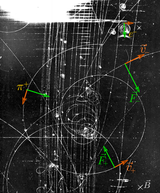
In physics, specifically in electromagnetism, the Lorentz force is the combination of electric and magnetic force on a point charge due to electromagnetic fields. A particle of charge q moving with a velocity v in an electric field E and a magnetic field B experiences a force of

<span class="mw-page-title-main">Maxwell's equations</span> Equations describing classical electromagnetism

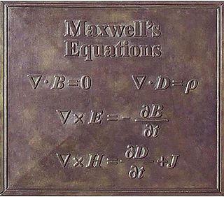
Maxwell's equations, or Maxwell–Heaviside equations, are a set of coupled partial differential equations that, together with the Lorentz force law, form the foundation of classical electromagnetism, classical optics, electric and magnetic circuits. The equations provide a mathematical model for electric, optical, and radio technologies, such as power generation, electric motors, wireless communication, lenses, radar, etc. They describe how electric and magnetic fields are generated by charges, currents, and changes of the fields. The equations are named after the physicist and mathematician James Clerk Maxwell, who, in 1861 and 1862, published an early form of the equations that included the Lorentz force law. Maxwell first used the equations to propose that light is an electromagnetic phenomenon. The modern form of the equations in their most common formulation is credited to Oliver Heaviside.

<span class="mw-page-title-main">Magnetic field</span> Distribution of magnetic force

A magnetic field is a physical field that describes the magnetic influence on moving electric charges, electric currents, and magnetic materials. A moving charge in a magnetic field experiences a force perpendicular to its own velocity and to the magnetic field. A permanent magnet's magnetic field pulls on ferromagnetic materials such as iron, and attracts or repels other magnets. In addition, a nonuniform magnetic field exerts minuscule forces on "nonmagnetic" materials by three other magnetic effects: paramagnetism, diamagnetism, and antiferromagnetism, although these forces are usually so small they can only be detected by laboratory equipment. Magnetic fields surround magnetized materials, electric currents, and electric fields varying in time. Since both strength and direction of a magnetic field may vary with location, it is described mathematically by a function assigning a vector to each point of space, called a vector field.

Flux describes any effect that appears to pass or travel through a surface or substance. Flux is a concept in applied mathematics and vector calculus which has many applications to physics. For transport phenomena, flux is a vector quantity, describing the magnitude and direction of the flow of a substance or property. In vector calculus flux is a scalar quantity, defined as the surface integral of the perpendicular component of a vector field over a surface.

<span class="mw-page-title-main">Electromagnetic induction</span> Production of voltage by a varying magnetic field

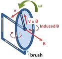
Electromagnetic or magnetic induction is the production of an electromotive force (emf) across an electrical conductor in a changing magnetic field.

<span class="mw-page-title-main">Magnetic flux</span> Surface integral of the magnetic field

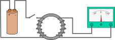
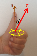
In physics, specifically electromagnetism, the magnetic flux through a surface is the surface integral of the normal component of the magnetic field B over that surface. It is usually denoted Φ or ΦB. The SI unit of magnetic flux is the weber, and the CGS unit is the maxwell. Magnetic flux is usually measured with a fluxmeter, which contains measuring coils, and it calculates the magnetic flux from the change of voltage on the coils.

<span class="mw-page-title-main">Electromotive force</span> Electrical action produced by a non-electrical source

In electromagnetism and electronics, electromotive force is an energy transfer to an electric circuit per unit of electric charge, measured in volts. Devices called electrical transducers provide an emf by converting other forms of energy into electrical energy. Other electrical equipment also produce an emf, such as batteries, which convert chemical energy, and generators, which convert mechanical energy. This energy conversion is achieved by physical forces applying physical work on electric charges. However, electromotive force itself is not a physical force, and ISO/IEC standards have deprecated the term in favor of source voltage or source tension instead.

<span class="mw-page-title-main">Inductance</span> Property of electrical conductors

Inductance is the tendency of an electrical conductor to oppose a change in the electric current flowing through it. The electric current produces a magnetic field around the conductor. The magnetic field strength depends on the magnitude of the electric current, and follows any changes in the magnitude of the current. From Faraday's law of induction, any change in magnetic field through a circuit induces an electromotive force (EMF) (voltage) in the conductors, a process known as electromagnetic induction. This induced voltage created by the changing current has the effect of opposing the change in current. This is stated by Lenz's law, and the voltage is called back EMF.

<span class="mw-page-title-main">Lenz's law</span> Electromagnetic opposition to change

Lenz's law states that the direction of the electric current induced in a conductor by a changing magnetic field is such that the magnetic field created by the induced current opposes changes in the initial magnetic field. It is named after physicist Heinrich Lenz, who formulated it in 1834.

<span class="mw-page-title-main">Ampère's circuital law</span> Concept in classical electromagnetism

In classical electromagnetism, Ampère's circuital law relates the circulation of a magnetic field around a closed loop to the electric current passing through the loop.

<span class="mw-page-title-main">Displacement current</span> Physical quantity in electromagnetism

In electromagnetism, displacement current density is the quantity D/∂t appearing in Maxwell's equations that is defined in terms of the rate of change of D, the electric displacement field. Displacement current density has the same units as electric current density, and it is a source of the magnetic field just as actual current is. However it is not an electric current of moving charges, but a time-varying electric field. In physical materials, there is also a contribution from the slight motion of charges bound in atoms, called dielectric polarization.

Kirchhoff's circuit laws are two equalities that deal with the current and potential difference in the lumped element model of electrical circuits. They were first described in 1845 by German physicist Gustav Kirchhoff. This generalized the work of Georg Ohm and preceded the work of James Clerk Maxwell. Widely used in electrical engineering, they are also called Kirchhoff's rules or simply Kirchhoff's laws. These laws can be applied in time and frequency domains and form the basis for network analysis.

"A Dynamical Theory of the Electromagnetic Field" is a paper by James Clerk Maxwell on electromagnetism, published in 1865. In the paper, Maxwell derives an electromagnetic wave equation with a velocity for light in close agreement with measurements made by experiment, and deduces that light is an electromagnetic wave.

<span class="mw-page-title-main">Circulation (physics)</span> Line integral of the fluid velocity around a closed curve

In physics, circulation is the line integral of a vector field around a closed curve. In fluid dynamics, the field is the fluid velocity field. In electrodynamics, it can be the electric or the magnetic field.

<span class="mw-page-title-main">Magnetic circuit</span> Closed loop path containing a magnetic flux

A magnetic circuit is made up of one or more closed loop paths containing a magnetic flux. The flux is usually generated by permanent magnets or electromagnets and confined to the path by magnetic cores consisting of ferromagnetic materials like iron, although there may be air gaps or other materials in the path. Magnetic circuits are employed to efficiently channel magnetic fields in many devices such as electric motors, generators, transformers, relays, lifting electromagnets, SQUIDs, galvanometers, and magnetic recording heads.

<span class="mw-page-title-main">Magnetic vector potential</span> Integral of the magnetic field

In classical electromagnetism, magnetic vector potential is the vector quantity defined so that its curl is equal to the magnetic field: . Together with the electric potential φ, the magnetic vector potential can be used to specify the electric field E as well. Therefore, many equations of electromagnetism can be written either in terms of the fields E and B, or equivalently in terms of the potentials φ and A. In more advanced theories such as quantum mechanics, most equations use potentials rather than fields.

<span class="mw-page-title-main">Faraday paradox</span> Apparent paradox with Faradays law of induction

The Faraday paradox or Faraday's paradox is any experiment in which Michael Faraday's law of electromagnetic induction appears to predict an incorrect result. The paradoxes fall into two classes:

<span class="mw-page-title-main">Maxwell stress tensor</span> Mathematical description in electromagnetism

The Maxwell stress tensor is a symmetric second-order tensor used in classical electromagnetism to represent the interaction between electromagnetic forces and mechanical momentum. In simple situations, such as a point charge moving freely in a homogeneous magnetic field, it is easy to calculate the forces on the charge from the Lorentz force law. When the situation becomes more complicated, this ordinary procedure can become impractically difficult, with equations spanning multiple lines. It is therefore convenient to collect many of these terms in the Maxwell stress tensor, and to use tensor arithmetic to find the answer to the problem at hand.

<span class="mw-page-title-main">Mathematical descriptions of the electromagnetic field</span> Formulations of electromagnetism

There are various mathematical descriptions of the electromagnetic field that are used in the study of electromagnetism, one of the four fundamental interactions of nature. In this article, several approaches are discussed, although the equations are in terms of electric and magnetic fields, potentials, and charges with currents, generally speaking.

The Maxwell-Lodge effect is a phenomenon of electromagnetic induction in which an electric charge, near a solenoid in which current changes slowly, feels an electromotive force (e.m.f.) even if the magnetic field is practically static inside and null outside. It can be considered a classical analogue of the quantum mechanical Aharonov–Bohm effect, where instead the field is exactly static inside and null outside.
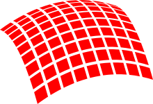
References

  1. Poyser, Arthur William (1892). Magnetism and Electricity: A manual for students in advanced classes. London and New York: Longmans, Green, & Co. Fig. 248, p. 245. Retrieved 2009-08-06.
  2. Sadiku, M. N. O. (2007). Elements of Electromagnetics (4th ed.). New York & Oxford: Oxford University Press. p. 386. ISBN   978-0-19-530048-2.
  3. "Applications of electromagnetic induction". Boston University. 1999-07-22.
  4. "A Brief History of Electromagnetism" (PDF).
  5. Ulaby, Fawwaz (2007). Fundamentals of applied electromagnetics (5th ed.). Pearson:Prentice Hall. p. 255. ISBN   978-0-13-241326-8.
  6. "Joseph Henry". Member Directory, National Academy of Sciences. Retrieved 2016-12-30.
  7. 1 2 Giancoli, Douglas C. (1998). Physics: Principles with Applications (5th ed.). pp.  623–624.
  8. 1 2 Faraday, Michael (1831-08-29). "Faraday's notebooks: Electromagnetic Induction" (PDF). The Royal Institution of Great Britain . Archived from the original (PDF) on 2021-08-30.
  9. Faraday, Michael; Day, P. (1999-02-01). The philosopher's tree: a selection of Michael Faraday's writings. CRC Press. p. 71. ISBN   978-0-7503-0570-9 . Retrieved 28 August 2011.
  10. 1 2 3 4 Williams, L. Pearce (1965). Michael Faraday . New York, Basic Books.[ full citation needed ]
  11. Clerk Maxwell, James (1904). A Treatise on Electricity and Magnetism. Vol. 2 (3rd ed.). Oxford University Press. pp. 178–179, 189.
  12. "Archives Biographies: Michael Faraday". The Institution of Engineering and Technology.
  13. Lenz, Emil (1834). "Ueber die Bestimmung der Richtung der durch elektodynamische Vertheilung erregten galvanischen Ströme". Annalen der Physik und Chemie. 107 (31): 483–494. Bibcode:1834AnP...107..483L. doi:10.1002/andp.18341073103.
    A partial translation of the paper is available in Magie, W. M. (1963). A Source Book in Physics. Cambridge, MA: Harvard Press. pp. 511–513.
  14. Siegel, Ethan (1 March 2019). "Relativity Wasn't Einstein's Miracle; It Was Waiting In Plain Sight For 71 Years". Forbes . Archived from the original on 3 July 2023. Retrieved 3 July 2023.
  15. Siegel, Ethan (28 June 2023). "71 years earlier, this scientist beat Einstein to relativity - Michael Faraday's 1834 law of induction was the key experiment behind the eventual discovery of relativity. Einstein admitted it himself". Big Think . Archived from the original on 28 June 2023. Retrieved 3 July 2023.
  16. Jordan, Edward; Balmain, Keith G. (1968). Electromagnetic Waves and Radiating Systems (2nd ed.). Prentice-Hall. p. 100. Faraday's Law, which states that the electromotive force around a closed path is equal to the negative of the time rate of change of magnetic flux enclosed by the path.
  17. Hayt, William (1989). Engineering Electromagnetics (5th ed.). McGraw-Hill. p.  312. ISBN   0-07-027406-1. The magnetic flux is that flux which passes through any and every surface whose perimeter is the closed path.
  18. 1 2 3 4 5 6 Feynman, Richard P. "The Feynman Lectures on Physics Vol. II". feynmanlectures.caltech.edu. Retrieved 2020-11-07.
  19. 1 2 Griffiths, David J. (1999). Introduction to Electrodynamics (3rd ed.). Upper Saddle River, NJ: Prentice Hall. pp.  301–303. ISBN   0-13-805326-X.
  20. Tipler; Mosca (2004). Physics for Scientists and Engineers. Macmillan. p. 795. ISBN   9780716708100.
  21. Neumann, Franz Ernst (1846). "Allgemeine Gesetze der inducirten elektrischen Ströme" (PDF). Annalen der Physik. 143 (1): 31–44. Bibcode:1846AnP...143...31N. doi:10.1002/andp.18461430103. Archived from the original (PDF) on 12 March 2020.
  22. 1 2 Yehuda Salu (2014). "A Left Hand Rule for Faraday's Law". The Physics Teacher . 52 (1): 48. Bibcode:2014PhTea..52...48S. doi:10.1119/1.4849156. Video Explanation
  23. Salu, Yehuda. "Bypassing Lenz's Rule - A Left Hand Rule for Faraday's Law". www.PhysicsForArchitects.com. Archived from the original on 7 May 2020. Retrieved 30 July 2017.
  24. Whelan, P. M.; Hodgeson, M. J. (1978). Essential Principles of Physics (2nd ed.). John Murray. ISBN   0-7195-3382-1.
  25. Nave, Carl R. "Faraday's Law". HyperPhysics. Georgia State University. Retrieved 2011-08-29.
  26. 1 2 Griffiths, David J. (2017). Introduction to Electrodynamics. 4 (Fourth ed.). Cambridge University Press. ISBN   978-1-108-42041-9. OCLC   965197645.
  27. Harrington, Roger F. (2003). Introduction to electromagnetic engineering. Mineola, NY: Dover Publications. p. 56. ISBN   0-486-43241-6.
  28. 1 2 Davison, M. E. (1973). "A Simple Proof that the Lorentz Force, Law Implied Faraday's Law of Induction, when B is Time Independent". American Journal of Physics. 41 (5): 713. Bibcode:1973AmJPh..41..713D. doi:10.1119/1.1987339.
  29. 1 2 Krey; Owen (14 August 2007). Basic Theoretical Physics: A Concise Overview. Springer. p. 155. ISBN   9783540368052.
  30. Simonyi, K. (1973). Theoretische Elektrotechnik (5th ed.). Berlin: VEB Deutscher Verlag der Wissenschaften. eq. 20, p. 47.
  31. 1 2 Stewart, Joseph V. Intermediate Electromagnetic Theory. p. 396. This example of Faraday's Law [the homopolar generator] makes it very clear that in the case of extended bodies care must be taken that the boundary used to determine the flux must not be stationary but must be moving with respect to the body.
  32. 1 2 Hughes, W. F.; Young, F. J. (1965). The Electromagnetodynamics of Fluid. John Wiley. Eq. (2.6–13) p. 53.
  33. Clerk Maxwell, James (1861). "On physical lines of force". Philosophical Magazine . 90. Taylor & Francis: 11–23. doi:10.1080/14786431003659180. S2CID   135524562.
  34. Griffiths, David J. (1999). Introduction to Electrodynamics (3rd ed.). Upper Saddle River, NJ: Prentice Hall. pp.  301–3. ISBN   0-13-805326-X.
    Note that the law relating flux to emf, which this article calls "Faraday's law", is referred to in Griffiths' terminology as the "universal flux rule". Griffiths uses the term "Faraday's law" to refer to what this article calls the "Maxwell–Faraday equation". So in fact, in the textbook, Griffiths' statement is about the "universal flux rule".
  35. The Feynman Lectures on Physics Vol. II Ch. 17: The Laws of Induction
  36. Fedosin, Sergey G. (2019). "On the Covariant Representation of Integral Equations of the Electromagnetic Field". Progress in Electromagnetics Research C. 96: 109–122. arXiv: 1911.11138 . Bibcode:2019arXiv191111138F. doi:10.2528/PIERC19062902. S2CID   208095922.
  37. Einstein, Albert. "On the Electrodynamics of Moving Bodies" (PDF).

Further reading