Metric connection

Last updated

In mathematics, a metric connection is a connection in a vector bundle E equipped with a bundle metric; that is, a metric for which the inner product of any two vectors will remain the same when those vectors are parallel transported along any curve. [1] This is equivalent to:

Contents

A special case of a metric connection is a Riemannian connection; there exists a unique such connection which is torsion free, the Levi-Civita connection. In this case, the bundle E is the tangent bundle TM of a manifold, and the metric on E is induced by a Riemannian metric on M.

Another special case of a metric connection is a Yang–Mills connection, which satisfies the Yang–Mills equations of motion. Most of the machinery of defining a connection and its curvature can be worked through without requiring any compatibility with the bundle metric. However, once one does require compatibility, this metric connection defines an inner product, Hodge star (which additionally needs a choice of orientation), and Laplacian, which are required to formulate the Yang–Mills equations.

Definition

Let be any local sections of the vector bundle E, and let X be a vector field on the base space M of the bundle. Let define a bundle metric, that is, a metric on the vector fibers of E. Then, a connection D on E is a metric connection if:

Here d is the ordinary differential of a scalar function. The covariant derivative can be extended so that it acts as a map on E-valued differential forms on the base space:

One defines for a function , and

where is a local smooth section for the vector bundle and is a (scalar-valued) p-form. The above definitions also apply to local smooth frames as well as local sections.

Metric versus dual pairing

The bundle metric imposed on E should not be confused with the natural pairing of a vector space and its dual, which is intrinsic to any vector bundle. The latter is a function on the bundle of endomorphisms so that

pairs vectors with dual vectors (functionals) above each point of M. That is, if is any local coordinate frame on E, then one naturally obtains a dual coordinate frame on E* satisfying .

By contrast, the bundle metric is a function on

giving an inner product on each vector space fiber of E. The bundle metric allows one to define an orthonormal coordinate frame by the equation

Given a vector bundle, it is always possible to define a bundle metric on it.

Following standard practice, [1] one can define a connection form, the Christoffel symbols and the Riemann curvature without reference to the bundle metric, using only the pairing They will obey the usual symmetry properties; for example, the curvature tensor will be anti-symmetric in the last two indices and will satisfy the second Bianchi identity. However, to define the Hodge star, the Laplacian, the first Bianchi identity, and the Yang–Mills functional, one needs the bundle metric. The Hodge star additionally needs a choice of orientation, and produces the Hodge dual of its argument.

Connection form

Given a local bundle chart, the covariant derivative can be written in the form

where A is the connection one-form.

A bit of notational machinery is in order. Let denote the space of differentiable sections on E, let denote the space of p-forms on M, and let be the endomorphisms on E. The covariant derivative, as defined here, is a map

One may express the connection form in terms of the connection coefficients as

The point of the notation is to distinguish the indices j, k, which run over the n dimensions of the fiber, from the index i, which runs over the m-dimensional base space. For the case of a Riemann connection below, the vector space E is taken to be the tangent bundle TM, and n = m.

The notation of A for the connection form comes from physics, in historical reference to the vector potential field of electromagnetism and gauge theory. In mathematics, the notation is often used in place of A, as in the article on the connection form; unfortunately, the use of for the connection form collides with the use of to denote a generic alternating form on the vector bundle.

Skew symmetry

The connection is skew-symmetric in the vector-space (fiber) indices; that is, for a given vector field , the matrix is skew-symmetric; equivalently, it is an element of the Lie algebra .

This can be seen as follows. Let the fiber be n-dimensional, so that the bundle E can be given an orthonormal local frame with i = 1, 2, ..., n. One then has, by definition, that , so that:

In addition, for each point of the bundle chart, the local frame is orthonormal:

It follows that, for every vector , that

That is, is skew-symmetric.

This is arrived at by explicitly using the bundle metric; without making use of this, and using only the pairing , one can only relate the connection form A on E to its dual A on E, as This follows from the definition of the dual connection as

Curvature

There are several notations in use for the curvature of a connection, including a modern one using F to denote the field strength tensor, a classical one using R as the curvature tensor, and the classical notation for the Riemann curvature tensor, most of which can be extended naturally to the case of vector bundles. None of these definitions require either a metric tensor, or a bundle metric, and can be defined quite concretely without reference to these. The definitions do, however, require a clear idea of the endomorphisms of E, as described above.

Compact style

The most compact definition of the curvature F is to define it as the 2-form taking values in , given by the amount by which the connection fails to be exact; that is, as

which is an element of

or equivalently,

To relate this to other common definitions and notations, let be a section on E. Inserting into the above and expanding, one finds

or equivalently, dropping the section

as a terse definition.

Component style

In terms of components, let where is the standard one-form coordinate bases on the cotangent bundle T*M. Inserting into the above, and expanding, one obtains (using the summation convention):

Keep in mind that for an n-dimensional vector space, each is an n×n matrix, the indices of which have been suppressed, whereas the indices i and j run over 1,...,m, with m being the dimension of the underlying manifold. Both of these indices can be made simultaneously manifest, as shown in the next section.

The notation presented here is that which is commonly used in physics; for example, it can be immediately recognizable as the gluon field strength tensor. For the abelian case, n=1, and the vector bundle is one-dimensional; the commutator vanishes, and the above can then be recognized as the electromagnetic tensor in more or less standard physics notation.

Relativity style

All of the indices can be made explicit by providing a smooth frame , i = 1, ..., n on . A given section then may be written as

In this local frame, the connection form becomes

with being the Christoffel symbol; again, the index i runs over 1, ..., m (the dimension of the underlying manifold M) while j and k run over 1, ..., n, the dimension of the fiber. Inserting and turning the crank, one obtains

where now identifiable as the Riemann curvature tensor. This is written in the style commonly employed in many textbooks on general relativity from the middle-20th century (with several notable exceptions, such as MTW, that pushed early on for an index-free notation). Again, the indices i and j run over the dimensions of the manifold M, while r and k run over the dimension of the fibers.

Tangent-bundle style

The above can be back-ported to the vector-field style, by writing as the standard basis elements for the tangent bundle TM. One then defines the curvature tensor as

so that the spatial directions are re-absorbed, resulting in the notation

Alternately, the spatial directions can be made manifest, while hiding the indices, by writing the expressions in terms of vector fields X and Y on TM. In the standard basis, X is

and likewise for Y. After a bit of plug and chug, one obtains

where

is the Lie derivative of the vector field Y with respect to X.

To recap, the curvature tensor maps fibers to fibers:

so that

To be very clear, are alternative notations for the same thing. Observe that none of the above manipulations ever actually required the bundle metric to go through. One can also demonstrate the second Bianchi identity

without having to make any use of the bundle metric.

Yang–Mills connection

The above development of the curvature tensor did not make any appeals to the bundle metric. That is, they did not need to assume that D or A were metric connections: simply having a connection on a vector bundle is sufficient to obtain the above forms. All of the different notational variants follow directly only from consideration of the endomorphisms of the fibers of the bundle.

The bundle metric is required to define the Hodge star and the Hodge dual; that is needed, in turn, to define the Laplacian, and to demonstrate that

Any connection that satisfies this identity is referred to as a Yang–Mills connection. It can be shown that this connection is a critical point of the Euler–Lagrange equations applied to the Yang–Mills action

where is the volume element, the Hodge dual of the constant 1. Note that three different inner products are required to construct this action: the metric connection on E, an inner product on End(E), equivalent to the quadratic Casimir operator (the trace of a pair of matricies), and the Hodge dual.

Riemannian connection

An important special case of a metric connection is a Riemannian connection. This is a connection on the tangent bundle of a pseudo-Riemannian manifold (M, g) such that for all vector fields X on M. Equivalently, is Riemannian if the parallel transport it defines preserves the metric g.

A given connection is Riemannian if and only if

for all vector fields X, Y and Z on M, where denotes the derivative of the function along this vector field .

The Levi-Civita connection is the torsion-free Riemannian connection on a manifold. It is unique by the fundamental theorem of Riemannian geometry. For every Riemannian connection, one may write a (unique) corresponding Levi-Civita connection. The difference between the two is given by the contorsion tensor.

In component notation, the covariant derivative is compatible with the metric tensor if

Although other covariant derivatives may be defined, usually one only considers the metric-compatible one. This is because given two covariant derivatives, and , there exists a tensor for transforming from one to the other:

If the space is also torsion-free, then the tensor is symmetric in its first two indices.

A word about notation

It is conventional to change notation and use the nabla symbol ∇ in place of D in this setting; in other respects, these two are the same thing. That is, ∇ = D from the previous sections above.

Likewise, the inner product on E is replaced by the metric tensor g on TM. This is consistent with historic usage, but also avoids confusion: for the general case of a vector bundle E, the underlying manifold M is not assumed to be endowed with a metric. The special case of manifolds with both a metric g on TM in addition to a bundle metric on E leads to Kaluza–Klein theory.

See also

Related Research Articles

In Riemannian or pseudo-Riemannian geometry, the Levi-Civita connection is the unique affine connection on the tangent bundle of a manifold that preserves the (pseudo-)Riemannian metric and is torsion-free.

<span class="mw-page-title-main">Differential operator</span> Typically linear operator defined in terms of differentiation of functions

In mathematics, a differential operator is an operator defined as a function of the differentiation operator. It is helpful, as a matter of notation first, to consider differentiation as an abstract operation that accepts a function and returns another function.

<span class="mw-page-title-main">Parallel transport</span> Construct in differential geometry

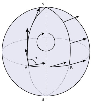
In geometry, parallel transport is a way of transporting geometrical data along smooth curves in a manifold. If the manifold is equipped with an affine connection, then this connection allows one to transport vectors of the manifold along curves so that they stay parallel with respect to the connection.

In mathematics, the Hodge star operator or Hodge star is a linear map defined on the exterior algebra of a finite-dimensional oriented vector space endowed with a nondegenerate symmetric bilinear form. Applying the operator to an element of the algebra produces the Hodge dual of the element. This map was introduced by W. V. D. Hodge.

In mathematics, a Lie algebroid is a vector bundle together with a Lie bracket on its space of sections and a vector bundle morphism , satisfying a Leibniz rule. A Lie algebroid can thus be thought of as a "many-object generalisation" of a Lie algebra.

In mathematics, and especially differential geometry and gauge theory, a connection on a fiber bundle is a device that defines a notion of parallel transport on the bundle; that is, a way to "connect" or identify fibers over nearby points. The most common case is that of a linear connection on a vector bundle, for which the notion of parallel transport must be linear. A linear connection is equivalently specified by a covariant derivative, an operator that differentiates sections of the bundle along tangent directions in the base manifold, in such a way that parallel sections have derivative zero. Linear connections generalize, to arbitrary vector bundles, the Levi-Civita connection on the tangent bundle of a pseudo-Riemannian manifold, which gives a standard way to differentiate vector fields. Nonlinear connections generalize this concept to bundles whose fibers are not necessarily linear.

In mathematics, the covariant derivative is a way of specifying a derivative along tangent vectors of a manifold. Alternatively, the covariant derivative is a way of introducing and working with a connection on a manifold by means of a differential operator, to be contrasted with the approach given by a principal connection on the frame bundle – see affine connection. In the special case of a manifold isometrically embedded into a higher-dimensional Euclidean space, the covariant derivative can be viewed as the orthogonal projection of the Euclidean directional derivative onto the manifold's tangent space. In this case the Euclidean derivative is broken into two parts, the extrinsic normal component and the intrinsic covariant derivative component.

<span class="mw-page-title-main">Affine connection</span> Construct allowing differentiation of tangent vector fields of manifolds

In differential geometry, an affine connection is a geometric object on a smooth manifold which connects nearby tangent spaces, so it permits tangent vector fields to be differentiated as if they were functions on the manifold with values in a fixed vector space. Connections are among the simplest methods of defining differentiation of the sections of vector bundles.

<span class="mw-page-title-main">Curvature of Riemannian manifolds</span>

In mathematics, specifically differential geometry, the infinitesimal geometry of Riemannian manifolds with dimension greater than 2 is too complicated to be described by a single number at a given point. Riemann introduced an abstract and rigorous way to define curvature for these manifolds, now known as the Riemann curvature tensor. Similar notions have found applications everywhere in differential geometry of surfaces and other objects. The curvature of a pseudo-Riemannian manifold can be expressed in the same way with only slight modifications.

In mathematics, and specifically differential geometry, a connection form is a manner of organizing the data of a connection using the language of moving frames and differential forms.

The contorsion tensor in differential geometry is the difference between a connection with and without torsion in it. It commonly appears in the study of spin connections. Thus, for example, a vielbein together with a spin connection, when subject to the condition of vanishing torsion, gives a description of Einstein gravity. For supersymmetry, the same constraint, of vanishing torsion, gives 11-dimensional supergravity. That is, the contorsion tensor, along with the connection, becomes one of the dynamical objects of the theory, demoting the metric to a secondary, derived role.

When studying and formulating Albert Einstein's theory of general relativity, various mathematical structures and techniques are utilized. The main tools used in this geometrical theory of gravitation are tensor fields defined on a Lorentzian manifold representing spacetime. This article is a general description of the mathematics of general relativity.

In mathematics, the Fubini–Study metric is a Kähler metric on a complex projective space CPn endowed with a Hermitian form. This metric was originally described in 1904 and 1905 by Guido Fubini and Eduard Study.

In mathematics—more specifically, in differential geometry—the musical isomorphism is an isomorphism between the tangent bundle and the cotangent bundle of a pseudo-Riemannian manifold induced by its metric tensor. There are similar isomorphisms on symplectic manifolds. The term musical refers to the use of the symbols (flat) and (sharp).

In mathematics, a vector-valued differential form on a manifold M is a differential form on M with values in a vector space V. More generally, it is a differential form with values in some vector bundle E over M. Ordinary differential forms can be viewed as R-valued differential forms.

In mathematics, a holomorphic vector bundle is a complex vector bundle over a complex manifold X such that the total space E is a complex manifold and the projection map π : EX is holomorphic. Fundamental examples are the holomorphic tangent bundle of a complex manifold, and its dual, the holomorphic cotangent bundle. A holomorphic line bundle is a rank one holomorphic vector bundle.

In Riemannian geometry and pseudo-Riemannian geometry, the Gauss–Codazzi equations are fundamental formulas which link together the induced metric and second fundamental form of a submanifold of a Riemannian or pseudo-Riemannian manifold.

In differential geometry, a fibered manifold is surjective submersion of smooth manifolds YX. Locally trivial fibered manifolds are fiber bundles. Therefore, a notion of connection on fibered manifolds provides a general framework of a connection on fiber bundles.

This article summarizes several identities in exterior calculus.

References

  1. 1 2 Jost, Jürgen (2011), Riemannian geometry and geometric analysis (PDF), Universitext (Sixth ed.), Springer, Heidelberg, doi:10.1007/978-3-642-21298-7, ISBN   978-3-642-21297-0, MR   2829653 .(Third edition: see chapter 3; Sixth edition: see chapter 4.)