
A centripetal force is a force that makes a body follow a curved path. The direction of the centripetal force is always orthogonal to the motion of the body and towards the fixed point of the instantaneous center of curvature of the path. Isaac Newton described it as "a force by which bodies are drawn or impelled, or in any way tend, towards a point as to a centre". In Newtonian mechanics, gravity provides the centripetal force causing astronomical orbits.
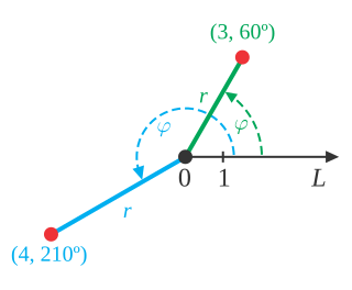
In mathematics, the polar coordinate system is a two-dimensional coordinate system in which each point on a plane is determined by a distance from a reference point and an angle from a reference direction. The reference point is called the pole, and the ray from the pole in the reference direction is the polar axis. The distance from the pole is called the radial coordinate, radial distance or simply radius, and the angle is called the angular coordinate, polar angle, or azimuth. Angles in polar notation are generally expressed in either degrees or radians.

In mathematics, a spherical coordinate system is a coordinate system for three-dimensional space where the position of a given point in space is specified by three numbers, : the radial distance of the radial liner connecting the point to the fixed point of origin ; the polar angle θ of the radial line r; and the azimuthal angle φ of the radial line r.

The Navier–Stokes equations are partial differential equations which describe the motion of viscous fluid substances. They were named after French engineer and physicist Claude-Louis Navier and the Irish physicist and mathematician George Gabriel Stokes. They were developed over several decades of progressively building the theories, from 1822 (Navier) to 1842–1850 (Stokes).
In mathematics, curvature is any of several strongly related concepts in geometry that intuitively measure the amount by which a curve deviates from being a straight line or by which a surface deviates from being a plane. If a curve or surface is contained in a larger space, curvature can be defined extrinsically relative to the ambient space. Curvature of Riemannian manifolds of dimension at least two can be defined intrinsically without reference to a larger space.

In physics, angular velocity, also known as angular frequency vector, is a pseudovector representation of how the angular position or orientation of an object changes with time, i.e. how quickly an object rotates around an axis of rotation and how fast the axis itself changes direction.
In the mathematical field of differential geometry, the Riemann curvature tensor or Riemann–Christoffel tensor is the most common way used to express the curvature of Riemannian manifolds. It assigns a tensor to each point of a Riemannian manifold. It is a local invariant of Riemannian metrics which measures the failure of the second covariant derivatives to commute. A Riemannian manifold has zero curvature if and only if it is flat, i.e. locally isometric to the Euclidean space. The curvature tensor can also be defined for any pseudo-Riemannian manifold, or indeed any manifold equipped with an affine connection.
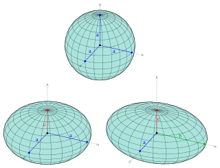
An ellipsoid is a surface that can be obtained from a sphere by deforming it by means of directional scalings, or more generally, of an affine transformation.

In fluid dynamics, the Euler equations are a set of quasilinear partial differential equations governing adiabatic and inviscid flow. They are named after Leonhard Euler. In particular, they correspond to the Navier–Stokes equations with zero viscosity and zero thermal conductivity.
In physics, the Hamilton–Jacobi equation, named after William Rowan Hamilton and Carl Gustav Jacob Jacobi, is an alternative formulation of classical mechanics, equivalent to other formulations such as Newton's laws of motion, Lagrangian mechanics and Hamiltonian mechanics.
In differential geometry, the four-gradient is the four-vector analogue of the gradient from vector calculus.

An osculating circle is a circle that best approximates the curvature of a curve at a specific point. It is tangent to the curve at that point and has the same curvature as the curve at that point. The osculating circle provides a way to understand the local behavior of a curve and is commonly used in differential geometry and calculus.
A theoretical motivation for general relativity, including the motivation for the geodesic equation and the Einstein field equation, can be obtained from special relativity by examining the dynamics of particles in circular orbits about the Earth. A key advantage in examining circular orbits is that it is possible to know the solution of the Einstein Field Equation a priori. This provides a means to inform and verify the formalism.
Bayesian linear regression is a type of conditional modeling in which the mean of one variable is described by a linear combination of other variables, with the goal of obtaining the posterior probability of the regression coefficients and ultimately allowing the out-of-sample prediction of the regressandconditional on observed values of the regressors. The simplest and most widely used version of this model is the normal linear model, in which given is distributed Gaussian. In this model, and under a particular choice of prior probabilities for the parameters—so-called conjugate priors—the posterior can be found analytically. With more arbitrarily chosen priors, the posteriors generally have to be approximated.

There are various mathematical descriptions of the electromagnetic field that are used in the study of electromagnetism, one of the four fundamental interactions of nature. In this article, several approaches are discussed, although the equations are in terms of electric and magnetic fields, potentials, and charges with currents, generally speaking.
In mathematics, the Möbius energy of a knot is a particular knot energy, i.e., a functional on the space of knots. It was discovered by Jun O'Hara, who demonstrated that the energy blows up as the knot's strands get close to one another. This is a useful property because it prevents self-intersection and ensures the result under gradient descent is of the same knot type.
Mechanics of planar particle motion is the analysis of the motion of particles gravitationally attracted to one another observed from non-inertial reference frames and the generalization of this problem to planetary motion. This type of analysis is closely related to centrifugal force, two-body problem, orbit and Kepler's laws of planetary motion. The mechanics of planar particle motion fall in the general field of analytical dynamics, and helps determine orbits from the given force laws. This article is focused more on the kinematic issues surrounding planar motion, which are the determination of the forces necessary to result in a certain trajectory given the particle trajectory.
In quantum mechanics, and especially quantum information theory, the purity of a normalized quantum state is a scalar defined as
In continuum mechanics, a compatible deformation tensor field in a body is that unique tensor field that is obtained when the body is subjected to a continuous, single-valued, displacement field. Compatibility is the study of the conditions under which such a displacement field can be guaranteed. Compatibility conditions are particular cases of integrability conditions and were first derived for linear elasticity by Barré de Saint-Venant in 1864 and proved rigorously by Beltrami in 1886.
Accelerations in special relativity (SR) follow, as in Newtonian Mechanics, by differentiation of velocity with respect to time. Because of the Lorentz transformation and time dilation, the concepts of time and distance become more complex, which also leads to more complex definitions of "acceleration". SR as the theory of flat Minkowski spacetime remains valid in the presence of accelerations, because general relativity (GR) is only required when there is curvature of spacetime caused by the energy–momentum tensor. However, since the amount of spacetime curvature is not particularly high on Earth or its vicinity, SR remains valid for most practical purposes, such as experiments in particle accelerators.


