Supply and demand

Last updated
Figure 1: The price P of a product is determined by a balance between production at each price (supply S) and the desires of those with purchasing power at each price (demand D). The diagram shows a positive shift in demand from D1 to D2, resulting in an increase in price (P) and quantity sold (Q) of the product. Supply-and-demand.svg
Figure 1: The price P of a product is determined by a balance between production at each price (supply S) and the desires of those with purchasing power at each price (demand D). The diagram shows a positive shift in demand from D1 to D2, resulting in an increase in price (P) and quantity sold (Q) of the product.
Supply and demand stacked in a conceptual chain Supply and demand-stacked4.png
Supply and demand stacked in a conceptual chain

In microeconomics, supply and demand is an economic model of price determination in a market. It postulates that, holding all else equal, in a competitive market, the unit price for a particular good or other traded item such as labor or liquid financial assets, will vary until it settles at a point where the quantity demanded will equal the quantity supplied (the market-clearing price), resulting in an economic equilibrium for price and quantity transacted. The concept of supply and demand forms the theoretical basis of modern economics.

Contents

In macroeconomics, as well, the aggregate demand-aggregate supply model has been used to depict how the quantity of total output and the aggregate price level may be determined in equilibrium.

Graphical representations

Supply schedule

A supply schedule, depicted graphically as a supply curve, is a table that shows the relationship between the price of a good and the quantity supplied by producers. Under the assumption of perfect competition, supply is determined by marginal cost: firms will produce additional output as long as the cost of producing an extra unit is less than the market price they receive.

A rise in the cost of raw materials would decrease supply, shifting the supply curve to the left because at each possible price a smaller quantity would be supplied. One may also think of this as a shift up in the supply curve, because the price must rise for producers to supply a given quantity. A fall in production costs would increase supply, shifting the supply curve to the right and down.

Mathematically, a supply curve is represented by a supply function, giving the quantity supplied as a function of its price and as many other variables as desired to better explain quantity supplied. The two most common specifications are:

1) linear supply function, e.g., the slanted line

, and

2) the constant-elasticity [1] supply function (also called isoelastic or log-log or loglinear supply function), e.g., the smooth curve

which can be rewritten as

By its very nature, the concept of a supply curve assumes that firms are perfect competitors, having no influence over the market price. This is because each point on the supply curve answers the question, "If this firm is faced with this potential price, how much output will it sell?" If a firm has market power—in violation of the perfect competitor model—its decision on how much output to bring to market influences the market price. Thus the firm is not "faced with" any given price, and a more complicated model, e.g., a monopoly or oligopoly or differentiated-product model, should be used.

Economists distinguish between the supply curve of an individual firm and the market supply curve. The market supply curve shows the total quantity supplied by all firms, so it is the sum of the quantities supplied by all suppliers at each potential price (that is, the individual firms' supply curves are added horizontally).

Economists distinguish between short-run and long-run supply curve. Short run refers to a time period during which one or more inputs are fixed (typically physical capital), and the number of firms in the industry is also fixed (if it is a market supply curve). Long run refers to a time period during which new firms enter or existing firms exit and all inputs can be adjusted fully to any price change. Long-run supply curves are flatter than short-run counterparts (with quantity more sensitive to price, more elastic supply).

Common determinants of supply are:

  1. Prices of inputs, including wages
  2. The technology used, productivity
  3. Firms' expectations about future prices
  4. Number of suppliers (for a market supply curve)

Demand schedule

A demand schedule, depicted graphically as a demand curve, represents the amount of a certain good that buyers are willing and able to purchase at various prices, assuming all other determinants of demand are held constant, such as income, tastes and preferences, and the prices of substitute and complementary goods. Generally, consumers will buy an additional unit as long as the marginal value of the extra unit is more than the market price they pay. According to the law of demand, the demand curve is always downward-sloping, meaning that as the price decreases, consumers will buy more of the good.

Mathematically, a demand curve is represented by a demand function, giving the quantity demanded as a function of its price and as many other variables as desired to better explain quantity demanded. The two most common specifications are linear demand, e.g., the slanted line

and the constant-elasticity demand function (also called isoelastic or log-log or loglinear demand function), e.g., the smooth curve

which can be rewritten as

As a matter of historical convention, a demand curve is drawn with price on the vertical y-axis and demand on the horizontal x-axis. In keeping with modern convention, a demand curve would instead be drawn with price on the x-axis and demand on the y-axis, because price is the independent variable and demand is the variable that is dependent upon price.

Just as the supply curve parallels the marginal cost curve, the demand curve parallels marginal utility, measured in dollars. [2] Consumers will be willing to buy a given quantity of a good, at a given price, if the marginal utility of additional consumption is equal to the opportunity cost determined by the price, that is, the marginal utility of alternative consumption choices. The demand schedule is defined as the willingness and ability of a consumer to purchase a given product at a certain time.

The demand curve is generally downward-sloping, but for some goods it is upward-sloping. Two such types of goods have been given definitions and names that are in common use: Veblen goods, goods which because of fashion or signalling are more attractive at higher prices, and Giffen goods, which, by virtue of being inferior goods that absorb a large part of a consumer's income (e.g., staples such as the classic example of potatoes in Ireland), may see an increase in quantity demanded when the price rises. The reason the law of demand is violated for Giffen goods is that the rise in the price of the good has a strong income effect, sharply reducing the purchasing power of the consumer so that he switches away from luxury goods to the Giffen good, e.g., when the price of potatoes rises, the Irish peasant can no longer afford meat and eats more potatoes to cover for the lost calories.

As with the supply curve, by its very nature the concept of a demand curve requires that the purchaser be a perfect competitor—that is, that the purchaser have no influence over the market price. This is true because each point on the demand curve answers the question, "If buyers are faced with this potential price, how much of the product will they purchase?" But, if a buyer has market power (that is, the amount he buys influences the price), he is not "faced with" any given price, and we must use a more complicated model, of monopsony.

As with supply curves, economists distinguish between the demand curve for an individual and the demand curve for a market. The market demand curve is obtained by adding the quantities from the individual demand curves at each price.

Common determinants of demand are:

  1. Income
  2. Tastes and preferences
  3. Prices of related goods and services
  4. Consumers' expectations about future prices and incomes
  5. Number of potential consumers
  6. Advertising

History of the curves

Cournotdemand.gif
Cournot's Recherches (1838)
Jenkincurves.gif
Jenkin's Graphical Representation (1870)
Marshalldemand.gif
Marshall's Principles (1890)
Figure 2. Early supply and demand curves

Since supply and demand can be considered as functions of price they have a natural graphical representation. Demand curves were first drawn by Augustin Cournot in his Recherches sur les Principes Mathématiques de la Théorie des Richesses (1838) – see Cournot competition. Supply curves were added by Fleeming Jenkin in The Graphical Representation of the Laws of Supply and Demand... of 1870. Both sorts of curve were popularised by Alfred Marshall who, in his Principles of Economics (1890), chose to represent price – normally the independent variable – by the vertical axis; a practice which remains common.

If supply or demand is a function of other variables besides price, it may be represented by a family of curves (with a change in the other variables constituting a shift between curves) or by a surface in a higher dimensional space.

Microeconomics

Figure 3: Supply and Demand Fig5 Supply and demand curves.jpg
Figure 3: Supply and Demand

Equilibrium

Generally speaking, an equilibrium is defined to be the price-quantity pair where the quantity demanded is equal to the quantity supplied. It is represented by the intersection of the demand and supply curves. The analysis of various equilibria is a fundamental aspect of microeconomics:

Market equilibrium: A situation in a market when the price is such that the quantity demanded by consumers is correctly balanced by the quantity that firms wish to supply. In this situation, the market clears. [3]

Changes in market equilibrium: Practical uses of supply and demand analysis often center on the different variables that change equilibrium price and quantity, represented as shifts in the respective curves. Comparative statics of such a shift traces the effects from the initial equilibrium to the new equilibrium.

Demand curve shifts:

When consumers increase the quantity demanded at a given price, it is referred to as an increase in demand. Increased demand can be represented on the graph as the curve being shifted to the right. At each price point, a greater quantity is demanded, as from the initial curve D1 to the new curve D2. In the diagram, this raises the equilibrium price from P1 to the higher P2. This raises the equilibrium quantity from Q1 to the higher Q2. (A movement along the curve is described as a "change in the quantity demanded" to distinguish it from a "change in demand", that is, a shift of the curve.) The increase in demand has caused an increase in (equilibrium) quantity. The increase in demand could come from changing tastes and fashions, incomes, price changes in complementary and substitute goods, market expectations, and number of buyers. This would cause the entire demand curve to shift changing the equilibrium price and quantity. Note in the diagram that the shift of the demand curve, by causing a new equilibrium price to emerge, resulted in movement along the supply curve from the point (Q1, P1) to the point (Q2, P2).

If the demand decreases, then the opposite happens: a shift of the curve to the left. If the demand starts at D2, and decreases to D1, the equilibrium price will decrease, and the equilibrium quantity will also decrease. The quantity supplied at each price is the same as before the demand shift, reflecting the fact that the supply curve has not shifted; but the equilibrium quantity and price are different as a result of the change (shift) in demand.

Supply curve shifts:

When technological progress occurs, the supply curve shifts. For example, assume that someone invents a better way of growing wheat so that the cost of growing a given quantity of wheat decreases. Otherwise stated, producers will be willing to supply more wheat at every price and this shifts the supply curve S1 outward, to S2—an increase in supply. This increase in supply causes the equilibrium price to decrease from P1 to P2. The equilibrium quantity increases from Q1 to Q2 as consumers move along the demand curve to the new lower price. As a result of a supply curve shift, the price and the quantity move in opposite directions. If the quantity supplied decreases, the opposite happens. If the supply curve starts at S2, and shifts leftward to S1, the equilibrium price will increase and the equilibrium quantity will decrease as consumers move along the demand curve to the new higher price and associated lower quantity demanded. The quantity demanded at each price is the same as before the supply shift, reflecting the fact that the demand curve has not shifted. But due to the change (shift) in supply, the equilibrium quantity and price have changed.

The movement of the supply curve in response to a change in a non-price determinant of supply is caused by a change in the y-intercept, the constant term of the supply equation. The supply curve shifts up and down the y axis as non-price determinants of demand change.

Partial equilibrium

Partial equilibrium, as the name suggests, takes into consideration only a part of the market to attain equilibrium.

Jain proposes (attributed to George Stigler): "A partial equilibrium is one which is based on only a restricted range of data, a standard example is price of a single product, the prices of all other products being held fixed during the analysis." [4]

The supply-and-demand model is a partial equilibrium model of economic equilibrium, where the clearance on the market of some specific goods is obtained independently from prices and quantities in other markets. In other words, the prices of all substitutes and complements, as well as income levels of consumers are constant. This makes analysis much simpler than in a general equilibrium model which includes an entire economy.

Here the dynamic process is that prices adjust until supply equals demand. It is a powerfully simple technique that allows one to study equilibrium, efficiency and comparative statics. The stringency of the simplifying assumptions inherent in this approach makes the model considerably more tractable, but may produce results which, while seemingly precise, do not effectively model real world economic phenomena.

Partial equilibrium analysis examines the effects of policy action in creating equilibrium only in that particular sector or market which is directly affected, ignoring its effect in any other market or industry assuming that they being small will have little impact if any.

Hence this analysis is considered to be useful in constricted markets.

Léon Walras first formalized the idea of a one-period economic equilibrium of the general economic system, but it was French economist Antoine Augustin Cournot and English political economist Alfred Marshall who developed tractable models to analyze an economic system.

Other markets

The model of supply and demand also applies to various specialty markets.

The model is commonly applied to wages, in the market for labor. The typical roles of supplier and demander are reversed. The suppliers are individuals, who try to sell their labor for the highest price. The demanders of labor are businesses, which try to buy the type of labor they need at the lowest price. The equilibrium price for a certain type of labor is the wage rate. [5] However, economist Steve Fleetwood revisited the empirical reality of supply and demand curves in labor markets and concluded that the evidence is "at best inconclusive and at worst casts doubt on their existence." For instance, he cites Kaufman and Hotchkiss (2006): "For adult men, nearly all studies find the labour supply curve to be negatively sloped or backward bending." [6]

In both classical and Keynesian economics, the money market is analyzed as a supply-and-demand system with interest rates being the price. The money supply may be a vertical supply curve, if the central bank of a country chooses to use monetary policy to fix its value regardless of the interest rate; in this case the money supply is totally inelastic. On the other hand, [7] the money supply curve is a horizontal line if the central bank is targeting a fixed interest rate and ignoring the value of the money supply; in this case the money supply curve is perfectly elastic. The demand for money intersects with the money supply to determine the interest rate. [8]

According to some studies, [9] the laws of supply and demand are applicable not only to the business relationships of people, but to the behaviour of social animals and to all living things that interact on the biological markets [10] in scarce resource environments.

The model of supply and demand accurately describes the characteristic of metabolic systems: specifically, it explains how feedback inhibition allows metabolic pathways to respond to the demand for a metabolic intermediates while minimizing effects due to variation in the supply. [11]

Empirical estimation

Demand and supply relations in a market can be statistically estimated from price, quantity, and other data with sufficient information in the model. This can be done with simultaneous-equation methods of estimation in econometrics. Such methods allow solving for the model-relevant "structural coefficients," the estimated algebraic counterparts of the theory. The Parameter identification problem is a common issue in "structural estimation." Typically, data on exogenous variables (that is, variables other than price and quantity, both of which are endogenous variables) are needed to perform such an estimation. An alternative to "structural estimation" is reduced-form estimation, which regresses each of the endogenous variables on the respective exogenous variables.

Macroeconomic uses

Human-hours worked per week in the United States. Labor is supply, money is demand Human hours worked per week.webp
Human-hours worked per week in the United States. Labor is supply, money is demand

Demand and supply have also been generalized to explain macroeconomic variables in a market economy, including the quantity of total output and the aggregate price level. The aggregate demand-aggregate supply model may be the most direct application of supply and demand to macroeconomics, but other macroeconomic models also use supply and demand. Compared to microeconomic uses of demand and supply, different (and more controversial) theoretical considerations apply to such macroeconomic counterparts as aggregate demand and aggregate supply. Demand and supply are also used in macroeconomic theory to relate money supply and money demand to interest rates, and to relate labor supply and labor demand to wage rates.

History

The 256th couplet of Tirukkural, which was composed at least 2000 years ago, says that "if people do not consume a product or service, then there will not be anybody to supply that product or service for the sake of price". [12]

According to Hamid S. Hosseini, the power of supply and demand was understood to some extent by several early Muslim scholars, such as fourteenth-century Syrian scholar Ibn Taymiyyah, who wrote: "If desire for goods increases while its availability decreases, its price rises. On the other hand, if availability of the good increases and the desire for it decreases, the price comes down." [13]

If desire for goods increases while its availability decreases, its price rises. On the other hand, if availability of the good increases and the desire for it decreases, the price comes down.

Adam Smith AdamSmith.jpg
Adam Smith

Shifting focus to the English etymology of the expression, it has been confirmed that the phrase 'supply and demand' was not used by English economics writers until after the end of the 17th century. [14] In John Locke's 1691 work Some Considerations on the Consequences of the Lowering of Interest and the Raising of the Value of Money, [15] Locke alluded to the idea of supply and demand, however, he failed to accurately label it as such and thus, he fell short in coining the phrase and conveying its true significance. [16] Locke wrote: “The price of any commodity rises or falls by the proportion of the number of buyer and sellers” and “that which regulates the price... [of goods] is nothing else but their quantity in proportion to [the] Vent.” [16] Locke's terminology drew criticism from John Law. Law argued that,"The Prices of Goods are not according to the quantity in proportion to the Vent, but in proportion to the Demand." [17] From Law the demand part of the phrase was given its proper title and it began to circulate among "prominent authorities" in the 1730s. [16] In 1755, Francis Hutcheson, in his A System of Moral Philosophy, furthered development toward the phrase by stipulating that, "the prices of goods depend on these two jointly, the Demand... and the Difficulty of acquiring." [16]

It was not until 1767 that the phrase "supply and demand" was first used by Scottish writer James Denham-Steuart in his Inquiry into the Principles of Political Economy. He originated the use of this phrase by effectively combining "supply" and "demand" together in a number of different occasions such as price determination and competitive analysis. In Steuart's chapter entitled "Of Demand", he argues that "The nature of Demand is to encourage industry; and when it is regularly made, the effect of it is, that the supply for the most part is found to be in proportion to it, and then the demand is simple". It is presumably from this chapter that the idea spread to other authors and economic thinkers. Adam Smith used the phrase after Steuart in his 1776 book The Wealth of Nations . In The Wealth of Nations, Smith asserted that the supply price was fixed but that its "merit" (value) would decrease as its "scarcity" increased, this idea by Smith was later named the law of demand. In 1803, Thomas Robert Malthus used the phrase "supply and demand" twenty times in the second edition of the Essay on Population. [16] And David Ricardo in his 1817 work, Principles of Political Economy and Taxation , titled one chapter, "On the Influence of Demand and Supply on Price". [18] In Principles of Political Economy and Taxation, Ricardo more rigorously laid down the idea of the assumptions that were used to build his ideas of supply and demand. In 1838, Antoine Augustin Cournot developed a mathematical model of supply and demand in his Researches into the Mathematical Principles of Wealth, it included diagrams. It is important to note that the use of the phrase was still rare and only a few examples of more than 20 uses in a single work have been identified by the end of the second decade of the 19th century. [16]

During the late 19th century the marginalist school of thought emerged. The main innovators of this approach were Stanley Jevons, Carl Menger, and Léon Walras. The key idea was that the price was set by the subjective value of a good at the margin. This was a substantial change from Adam Smith's thoughts on determining the supply price.

In his 1870 essay "On the Graphical Representation of Supply and Demand", Fleeming Jenkin in the course of "introduc[ing] the diagrammatic method into the English economic literature" published the first drawing of supply and demand curves in English, [19] including comparative statics from a shift of supply or demand and application to the labor market. [20] The model was further developed and popularized by Alfred Marshall in the 1890 textbook Principles of Economics . [18]

Criticism

The philosopher Hans Albert has argued that the ceteris paribus conditions of the marginalist theory rendered the theory itself an empty tautology and completely closed to experimental testing. In essence, he argues, the supply and demand curves (theoretical functions which express the quantity of a product which would be offered or requested for a given price) are purely ontological.[ citation needed ] [21]

Piero Sraffa's critique focused on the inconsistency (except in implausible circumstances) of partial equilibrium analysis and the rationale for the upward slope of the supply curve in a market for a produced consumption good. [22] The notability of Sraffa's critique is also demonstrated by Paul Samuelson's comments and engagements with it over many years, for example:

What a cleaned-up version of Sraffa (1926) establishes is how nearly empty are all of Marshall's partial equilibrium boxes. To a logical purist of Wittgenstein and Sraffa class, the Marshallian partial equilibrium box of constant cost is even more empty than the box of increasing cost. [23]

Modern Post-Keynesians criticize the supply and demand model for failing to explain the prevalence of administered prices, in which retail prices are set by firms, primarily based on a mark-up over normal average unit costs, and are not responsive to changes in demand up to capacity. [24]

Some economists criticize the conventional supply and demand theory for failing to explain or anticipate asset bubbles that can arise from a positive feedback loop. [25] Conventional supply and demand theory assumes that expectations of consumers do not change as a consequence of price changes. In scenarios such as the United States housing bubble, an initial price change of an asset can increase the expectations of investors, making the asset more lucrative and contributing to further price increases until market sentiment changes, which creates a positive feedback loop and an asset bubble. [26] Asset bubbles cannot be understood in the conventional supply and demand framework because the conventional system assumes a price change will be self-correcting and the system will snap back to equilibrium.

Paul Cockshott's critique focuses on the unfalsifiability of the neoclassical model. In the linear examples given above we have four unknowns: the slope and intercept of both the supply curve and the demand curve. But because we only have two knowns, price and quantity, any set of supply and demand curves that crosses the point could explain the data. Hence unfalsifiability. Cockshott also points out that prices are negatively correlated with quantity due to economies of scale, not positively correlated as the theory suggests. Finally, Cockshott argues that the theory is needlessly complicated when compared to the labour theory of value, and that having to introduce a notion of the curves shifting amounts to adding epicycles. [27]

See also

Related Research Articles

<span class="mw-page-title-main">Microeconomics</span> Behavior of individuals and firms

Microeconomics is a branch of economics that studies the behavior of individuals and firms in making decisions regarding the allocation of scarce resources and the interactions among these individuals and firms. Microeconomics focuses on the study of individual markets, sectors, or industries as opposed to the national economy as a whole, which is studied in macroeconomics.

<span class="mw-page-title-main">Macroeconomics</span> Study of an economy as a whole

Macroeconomics is a branch of economics that deals with the performance, structure, behavior, and decision-making of an economy as a whole. This includes regional, national, and global economies. Macroeconomists study topics such as output/GDP and national income, unemployment, price indices and inflation, consumption, saving, investment, energy, international trade, and international finance.

In economics, specifically general equilibrium theory, a perfect market, also known as an atomistic market, is defined by several idealizing conditions, collectively called perfect competition, or atomistic competition. In theoretical models where conditions of perfect competition hold, it has been demonstrated that a market will reach an equilibrium in which the quantity supplied for every product or service, including labor, equals the quantity demanded at the current price. This equilibrium would be a Pareto optimum.

In economics, general equilibrium theory attempts to explain the behavior of supply, demand, and prices in a whole economy with several or many interacting markets, by seeking to prove that the interaction of demand and supply will result in an overall general equilibrium. General equilibrium theory contrasts with the theory of partial equilibrium, which analyzes a specific part of an economy while its other factors are held constant. In general equilibrium, constant influences are considered to be noneconomic, or in other words, considered to be beyond the scope of economic analysis. The noneconomic influences may change given changes in the economic factors however, and therefore the prediction accuracy of an equilibrium model may depend on the independence of the economic factors from noneconomic ones.

<span class="mw-page-title-main">Economic surplus</span> Concept in economics

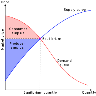
In mainstream economics, economic surplus, also known as total welfare or total social welfare or Marshallian surplus, is either of two related quantities:

<span class="mw-page-title-main">IS–LM model</span> Macroeconomic model relating interest rates and asset market

The IS–LM model, or Hicks–Hansen model, is a two-dimensional macroeconomic model which is used as a pedagogical tool in macroeconomic teaching. The IS–LM model shows the relationship between interest rates and output in the short run in a closed economy. The intersection of the "investment–saving" (IS) and "liquidity preference–money supply" (LM) curves illustrates a "general equilibrium" where supposed simultaneous equilibria occur in both the goods and the money markets. The IS–LM model shows the importance of various demand shocks on output and consequently offers an explanation of changes in national income in the short run when prices are fixed or sticky. Hence, the model can be used as a tool to suggest potential levels for appropriate stabilisation policies. It is also used as a building block for the demand side of the economy in more comprehensive models like the AD–AS model.

This aims to be a complete article list of economics topics:

In economics, elasticity measures the responsiveness of one economic variable to a change in another. If the price elasticity of the demand of something is -2, a 10% increase in price causes the quantity demanded to fall by 20%. Elasticity in economics provides an understanding of changes in the behavior of the buyers and sellers with price changes. There are two types of elasticity for demand and supply, one is inelastic demand and supply and the other one is elastic demand and supply.

In economics, economic equilibrium is a situation in which economic forces such as supply and demand are balanced and in the absence of external influences the values of economic variables will not change. For example, in the standard text perfect competition, equilibrium occurs at the point at which quantity demanded and quantity supplied are equal.

In economics, aggregate demand (AD) or domestic final demand (DFD) is the total demand for final goods and services in an economy at a given time. It is often called effective demand, though at other times this term is distinguished. This is the demand for the gross domestic product of a country. It specifies the amount of goods and services that will be purchased at all possible price levels. Consumer spending, investment, corporate and government expenditure, and net exports make up the aggregate demand.

In economics, effective demand (ED) in a market is the demand for a product or service which occurs when purchasers are constrained in a different market. It contrasts with notional demand, which is the demand that occurs when purchasers are not constrained in any other market. In the aggregated market for goods in general, demand, notional or effective, is referred to as aggregate demand. The concept of effective supply parallels the concept of effective demand. The concept of effective demand or supply becomes relevant when markets do not continuously maintain equilibrium prices.

<span class="mw-page-title-main">Demand curve</span> Graph of how much of something a consumer would buy at a certain price

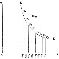
A demand curve is a graph depicting the inverse demand function, a relationship between the price of a certain commodity and the quantity of that commodity that is demanded at that price. Demand curves can be used either for the price-quantity relationship for an individual consumer, or for all consumers in a particular market.

In economics, tax incidence or tax burden is the effect of a particular tax on the distribution of economic welfare. Economists distinguish between the entities who ultimately bear the tax burden and those on whom the tax is initially imposed. The tax burden measures the true economic effect of the tax, measured by the difference between real incomes or utilities before and after imposing the tax, and taking into account how the tax causes prices to change. For example, if a 10% tax is imposed on sellers of butter, but the market price rises 8% as a result, most of the tax burden is on buyers, not sellers. The concept of tax incidence was initially brought to economists' attention by the French Physiocrats, in particular François Quesnay, who argued that the incidence of all taxation falls ultimately on landowners and is at the expense of land rent. Tax incidence is said to "fall" upon the group that ultimately bears the burden of, or ultimately suffers a loss from, the tax. The key concept of tax incidence is that the tax incidence or tax burden does not depend on where the revenue is collected, but on the price elasticity of demand and price elasticity of supply. As a general policy matter, the tax incidence should not violate the principles of a desirable tax system, especially fairness and transparency. The concept of tax incidence is used in political science and sociology to analyze the level of resources extracted from each income social stratum in order to describe how the tax burden is distributed among social classes. That allows one to derive some inferences about the progressive nature of the tax system, according to principles of vertical equity.

In economics, the long-run is a theoretical concept in which all markets are in equilibrium, and all prices and quantities have fully adjusted and are in equilibrium. The long-run contrasts with the short-run, in which there are some constraints and markets are not fully in equilibrium. More specifically, in microeconomics there are no fixed factors of production in the long-run, and there is enough time for adjustment so that there are no constraints preventing changing the output level by changing the capital stock or by entering or leaving an industry. This contrasts with the short-run, where some factors are variable and others are fixed, constraining entry or exit from an industry. In macroeconomics, the long-run is the period when the general price level, contractual wage rates, and expectations adjust fully to the state of the economy, in contrast to the short-run when these variables may not fully adjust.

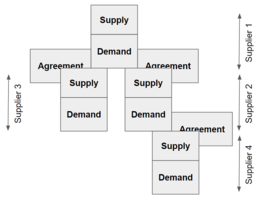
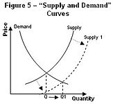
In economics, demand is the quantity of a good that consumers are willing and able to purchase at various prices during a given time. The relationship between price and quantity demand is also called the demand curve. Demand for a specific item is a function of an item's perceived necessity, price, perceived quality, convenience, available alternatives, purchasers' disposable income and tastes, and many other options.

<span class="mw-page-title-main">Supply (economics)</span> Amount of a good that sellers are willing to provide in the market

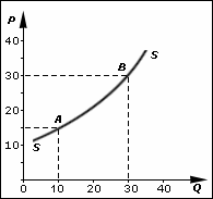
In economics, supply is the amount of a resource that firms, producers, labourers, providers of financial assets, or other economic agents are willing and able to provide to the marketplace or to an individual. Supply can be in produced goods, labour time, raw materials, or any other scarce or valuable object. Supply is often plotted graphically as a supply curve, with the price per unit on the vertical axis and quantity supplied as a function of price on the horizontal axis. This reversal of the usual position of the dependent variable and the independent variable is an unfortunate but standard convention.

The neoclassical synthesis (NCS), neoclassical–Keynesian synthesis, or just neo-Keynesianism was a neoclassical economics academic movement and paradigm in economics that worked towards reconciling the macroeconomic thought of John Maynard Keynes in his book The General Theory of Employment, Interest and Money (1936). It was formulated most notably by John Hicks (1937), Franco Modigliani (1944), and Paul Samuelson (1948), who dominated economics in the post-war period and formed the mainstream of macroeconomic thought in the 1950s, 60s, and 70s.

<span class="mw-page-title-main">AD–AS model</span> Macroeconomic model relating aggregate demand and supply

The AD–AS or aggregate demand–aggregate supply model is a widely used macroeconomic model that explains short-run and long-run economic changes through the relationship of aggregate demand (AD) and aggregate supply (AS) in a diagram. It coexists in an older and static version depicting the two variables output and price level, and in a newer dynamic version showing output and inflation.

<span class="mw-page-title-main">History of macroeconomic thought</span>

Macroeconomic theory has its origins in the study of business cycles and monetary theory. In general, early theorists believed monetary factors could not affect real factors such as real output. John Maynard Keynes attacked some of these "classical" theories and produced a general theory that described the whole economy in terms of aggregates rather than individual, microeconomic parts. Attempting to explain unemployment and recessions, he noticed the tendency for people and businesses to hoard cash and avoid investment during a recession. He argued that this invalidated the assumptions of classical economists who thought that markets always clear, leaving no surplus of goods and no willing labor left idle.

This glossary of economics is a list of definitions of terms and concepts used in economics, its sub-disciplines, and related fields.

References

  1. The elasticity coefficient, or often just elasticity, is an important parameter in metabolic control analysis, used to express the local response of an enzyme or other chemical reaction to changes in its environment.
  2. "Marginal Utility and Demand" . Retrieved 2007-02-09.
  3. Mankiw, N.G.; Taylor, M.P. (2011). Economics (2nd ed., revised ed.). Andover: Cengage Learning.
  4. Jain, T.R. (2006–2007). Microeconomics and Basic Mathematics. New Delhi: VK Publications. p. 28. ISBN   978-81-87140-89-4.
  5. Kibbe, Matthew B. "The Minimum Wage: Washington's Perennial Myth". Cato Institute . Retrieved 2007-02-09.
  6. Fleetwood, Steve (August 2014). "Do labour supply and demand curves exist?". Cambridge Journal of Economics. 38 (5): 1087–113. doi:10.1093/cje/beu003.
  7. Basij J. Moore, Horizontalists and Verticalists: The Macroeconomics of Credit Money, Cambridge University Press, 1988
  8. Ritter, Lawrence S.; Silber, William L.; Udell, Gregory F. (2000). Principles of Money, Banking, and Financial Markets (10th ed.). Addison-Wesley, Menlo Park C. pp. 431–38, 465–76. ISBN   978-0-321-37557-5.
  9. Velev, Milen V. Entropy and free-energy based interpretation of the laws of supply and demand. SN Bus Econ 1, 1 (2021). https://doi.org/10.1007/s43546-020-00009-6
  10. Noë, R., Hammerstein, P. Biological markets: supply and demand determine the effect of partner choice in cooperation, mutualism and mating. Behav Ecol Sociobiol 35, 1–11 (1994). https://doi.org/10.1007/BF00167053
  11. Hofmeyr, J.-H.S.; Cornish-Bowden, A. (2000). "Regulating the cellular economy of supply and demand". FEBS Lett. 476 (1): 47–51. doi:10.1111/j.1432-1033.1991.tb21071.x. PMID   1879427.
  12. C Chendroyaperumal (2010). The First Laws in Economics and Indian Economic Thought – Thirukkural
  13. 1 2 Hosseini, Hamid S. (2003). "Contributions of Medieval Muslim Scholars to the History of Economics and their Impact: A Refutation of the Schumpeterian Great Gap". In Biddle, Jeff E.; Davis, Jon B.; Samuels, Warren J. (eds.). A Companion to the History of Economic Thought. Malden, MA: Blackwell. pp. 28–45 [28 & 38]. doi:10.1002/9780470999059.ch3. ISBN   978-0-631-22573-7. (citing Hamid S. Hosseini, 1995. "Understanding the Market Mechanism Before Adam Smith: Economic Thought in Medieval Islam," History of Political Economy, Vol. 27, No. 3, 539–61).
  14. Thweatt, W.O. (1983). "Origins of the terminology, supply and demand". Scottish Journal of Political Economy. 30 (3): 287–294. doi:10.1111/j.1467-9485.1983.tb01020.x.
  15. John Locke (1691) Some Considerations on the consequences of the Lowering of Interest and the Raising of the Value of Money
  16. 1 2 3 4 5 6 Groenewegen P. (2008) ‘Supply and Demand’. In: Palgrave Macmillan (eds) The New Palgrave Dictionary of Economics. Palgrave Macmillan, London
  17. Law, J. (1705). Money and Trade Considered with a Proposal for Supplying the Nation with Money. Edinburgh: Anderson.
  18. 1 2 Humphrey, Thomas M. (1992). "Marshallian Cross Diagrams and their Uses before Alfred Marshall" (PDF). Economic Review (Mar/Apr): 3–23. Retrieved 2019-07-27.
  19. A.D. Brownlie and M. F. Lloyd Prichard, 1963. "Professor Fleeming Jenkin, 1833–1885 Pioneer in Engineering and Political Economy," Oxford Economic Papers, NS, 15(3), p. 211.
  20. Fleeming Jenkin, 1870. "The Graphical Representation of the Laws of Supply and Demand, and their Application to Labour," in Alexander Grant, ed., (Scroll to chapter) Recess Studies, ch. VI, pp. 151–85. Edinburgh: Edmonston and Douglas
  21. Albert, Hans (1963). "Model Platonism: Neoclassical economic thought in critical light (Der neoklassische Stil des ökonomischen Denkens in kritischer Beleuchtung)". Cambridge.org.
  22. Avi J. Cohen, "'The Laws of Returns Under Competitive Conditions': Progress in Microeconomics Since Sraffa (1926)?", Eastern Economic Journal, V. 9, N. 3 (Jul.-Sep.): 1983)
  23. Paul A. Samuelson, "Reply" in Critical Essays on Piero Sraffa's Legacy in Economics (edited by H. D. Kurz) Cambridge University Press, 2000
  24. Lee, F. S. (1999). Post Keynesian price theory. Cambridge University Press.
  25. What Every Economics Student Needs to Know and Doesn't Get in the Usual Principles Text. Routledge. 2014. pp. 55, 66, 244.
  26. "Positive Feedback". Investopedia. Retrieved November 13, 2018.
  27. Paul Cockshott: How the World Works: The Story of Human Labor from Prehistory to the Modern Day. Monthly Review Press, 2020, ISBN   978-1-58367-777-3. pp. 65-68

Further reading