3D sound localization

Last updated

3D sound localization refers to an acoustic technology that is used to locate the source of a sound in a three-dimensional space. The source location is usually determined by the direction of the incoming sound waves (horizontal and vertical angles) and the distance between the source and sensors. It involves the structure arrangement design of the sensors and signal processing techniques.

Contents

Most mammals (including humans) use binaural hearing to localize sound, by comparing the information received from each ear in a complex process that involves a significant amount of synthesis. It is difficult to localize using monaural hearing, especially in 3D space.

Technology

Sound localization technology is used in some audio and acoustics fields, such as hearing aids, surveillance [1] and navigation. Existing real-time passive sound localization systems are mainly based on the time-difference-of-arrival (TDOA) approach, limiting sound localization to two-dimensional space, and are not practical in noisy conditions.

Applications

Collecting Multibeam Sonar Data Collecting Multibeam Sonar Data.jpg
Collecting Multibeam Sonar Data

Applications of sound source localization include sound source separation, sound source tracking, and speech enhancement. Sonar uses sound source localization techniques to identify the location of a target. 3D sound localization is also used for effective human-robot interaction. With the increasing demand for robotic hearing, some applications of 3D sound localization such as human-machine interface, handicapped aid, and military applications, are being explored. [2]

Cues for sound localization

Localization cues [3] are features that help localize sound. Cues for sound localization include binaural and monoaural cues.

How does one localize sound?

The first clue our hearing uses is interaural time difference. Sound from a source directly in front of or behind us will arrive simultaneously at both ears. If the source moves to the left or right, our ears pick up the sound from the same source arriving at both ears - but with a certain delay. Another way of saying it could be, that the two ears pick up different phases of the same signal. [4]

Methods

There are many different methods of 3D sound localization. For instance:

Steered Beamformer Approach

This approach utilizes eight microphones combined with a steered beamformer enhanced by the Reliability Weighted Phase Transform (RWPHAT). The final results are filtered through a particle filter that tracks sources and prevents false directions.

The motivation of using this method is that based on previous research. This method is used for multiple sound source tracking and localizing despite soundtracking and localization only apply for a single sound source.

Beamformer-based Sound Localization

To maximize the output energy of a delay-and-sum beamformer in order to find the maximum value of the output of a beamformer steered in all possible directions. Using the Reliability Weighted Phase Transform (RWPHAT) method, The output energy of M-microphone delay-and-sum beamformer is

Where E indicates the energy, and K is a constant, is the microphone pairs cross-correlation defined by Reliability Weighted Phase Transform:

the weighted factor reflect the reliability of each frequency component, and defined as the Wiener Filter gain , where is an estimate of a prior SNR at microphone, at time frame , for frequency , computed using the decision-directed approach. [8]

The is the signal from microphone and is the delay of arrival for that microphone. The more specific procedure of this method is proposed by Valin and Michaud [9]

The advantage of this method is that it detects the direction of the sound and derives the distance of sound sources. The main drawback of the beamforming approach is the imperfect nature of sound localization accuracy and capability, versus the neural network approach, which uses moving speakers.

Collocated Microphone Array Approach

This method relates to the technique of Real-Time sound localization utilizing an Acoustic Vector Sensor (AVS) array, which measures all three components of the acoustic particle velocity, as well as the sound pressure, unlike conventional acoustic sensor arrays that only utilize the pressure information and delays in the propagating acoustic field. Exploiting this extra information, AVS arrays are able to significantly improve the accuracy of source localization.

Acoustic Vector Array

Picture of a 3D Acoustic Vector Sensor (air) Acoustic Vector Sensor.jpg
Picture of a 3D Acoustic Vector Sensor (air)

• Contains three orthogonally placed acoustic particle velocity sensors (shown as X, Y and Z array) and one omnidirectional acoustic microphone (O).

• Commonly used both in air [10] and underwater.

• Can be used in combination with the Offline Calibration Process [11] to measure and interpolate the impulse response of X, Y, Z and O arrays, to obtain their steering vector.

A sound signal is first windowed using a rectangular window, then each resulting segment signal is created as a frame. 4 parallel frames are detected from XYZO array and used for DOA estimation. The 4 frames are split into small blocks with equal size, then the Hamming window and FFT are used to convert each block from a time domain to a frequency domain. Then the output of this system is represented by a horizontal angle and a vertical angle of the sound sources which is found by the peak in the combined 3D spatial spectrum.

The advantages of this array, compared with past microphone array, are that this device has a high performance even if the aperture is small, and it can localize multiple low frequency and high frequency wide band sound sources simultaneously. Applying an O array can make more available acoustic information, such as amplitude and time difference. Most importantly, XYZO array has a better performance with a tiny size.

The AVS is one kind of collocated multiple microphone array, it makes use of a multiple microphone array approach for estimating the sound directions by multiple arrays and then finds the locations by using reflection information such as where the direction is detected where different arrays cross.

Motivation of the Advanced Microphone array

Sound reflections always occur in an actual environment and microphone arrays [12] cannot avoid observing those reflections. This multiple array approach was tested using fixed arrays in the ceiling; the performance of the moving scenario still need to be tested.

Learning how to apply Multiple Microphone Array

Angle uncertainty (AU) will occur when estimating direction, and position uncertainty (PU) will also aggravate with increasing distance between the array and the source. We know that:

Where r is the distance between array center to source, and AU is angle uncertainly. Measurement is used for judging whether two directions cross at some location or not. Minimum distance between two lines:

whereand are two directions, are vectors parallel to detected direction, and are the position of arrays.

If

Two lines are judged as crossing. When two lines are crossing, we can compute the sound source location using the following:

is the estimation of sound source position, is the position where each direction intersect the line with minimum distance, and is the weighted factors. As the weighting factor , we determined use or from the array to the line with minimum distance.

Scanning Techniques

3D sound localization of a large compressor 3D sound localization of a large compressor.png
3D sound localization of a large compressor

Scan-based techniques are a powerful tool for localizing and visualizing time-stationary sound sources, as they only require the use of a single sensor and a position tracking system. One popular method for achieving this is through the use of an Acoustic Vector Sensor (AVS), also known as a 3D Sound Intensity Probe, in combination with a 3D tracker.

The measurement procedure involves manually moving the AVS sensor around the sound source while a stereo camera is used to extract the instantaneous position of the sensor in three-dimensional space. The recorded signals are then split into multiple segments and assigned to a set of positions using a spatial discretization algorithm. This allows for the computation of a vector representation of the acoustic variations across the sound field, using combinations of the sound pressure and the three orthogonal acoustic particle velocities.

The results of the AVS analysis can be presented over a 3D sketch of the tested object, providing a visual representation of the sound distribution around a 3D mesh of the object or environment. This can be useful for localizing sound sources in a variety of fields, such as architectural acoustics, noise control, and audio engineering, as it allows for a detailed understanding of the sound distribution and its interactions with the surrounding environment.

Learning method for binaural hearing

Structure of the binaural robot dummy head Binaural robot head2.png
Structure of the binaural robot dummy head

Binaural hearing learning [5] is a bionic method. The sensor is a robot dummy head with 2 sensor microphones along with the artificial pinna (reflector). The robot head has 2 rotation axes and can rotate horizontally and vertically. The reflector causes the spectrum change into a certain pattern for incoming white noise sound wave and this pattern is used for the cue of the vertical localization. The cue for horizontal localization is ITD. The system makes use of a learning process using neural networks by rotating the head with a settled white noise sound source and analyzing the spectrum. Experiments show that the system can identify the direction of the source well in a certain range of angle of arrival. It cannot identify the sound coming outside the range due to the collapsed spectrum pattern of the reflector. Binaural hearing use only 2 microphones and is capable of concentrating on one source among multiple sources of noises.

In the real sound localization, the robot head and the torso play a functional role, in addition to the two pinnae. This functions as spatial linear filtering and the filtering is always quantified in terms of Head-Related Transfer Function (HRTF). [14] HRTF also uses the robot head sensor, which is the binaural hearing model. The HRTF can be derived based on various cues for localization. Sound localization with HRTF is filtering the input signal with a filter which is designed based on the HRTF. Instead of using the neural networks, a head-related transfer function is used and the localization is based on a simple correlation approach.

See more: Head-related transfer function.

Cross-power spectrum phase (CSP) analysis

CSP method [15] is also used for the binaural model. The idea is that the angle of arrival can be derived through the time delay of arrival (TDOA) between two microphones, and TDOA can be estimated by finding the maximum coefficients of CSP. CSP coefficients are derived by:

Where and are signals entering the microphone and respectively
Time delay of arrival() then can be estimated by:

Sound source direction is

Where is the sound propagation speed, is the sampling frequency and is the distance with maximum time delay between 2 microphones.

CPS method does not require the system impulse response data that HRTF needs. An expectation-maximization algorithm is also used for localizing several sound sources and reduce the localization errors. The system is capable of identifying several moving sound source using only two microphones.

2D sensor line array

Demonstration of 2d line sensor array 2D array demo3.png
Demonstration of 2d line sensor array

In order to estimate the location of a source in 3D space, two line sensor arrays can be placed horizontally and vertically. An example is a 2D line array used for underwater source localization. [16] By processing the data from two arrays using the maximum likelihood method, the direction, range and depth of the source can be identified simultaneously. Unlike the binaural hearing model, this method is similar to the spectral analysis method. The method can be used to localize a distant source.

Self-rotating Bi-Microphone Array

The rotation of the two-microphone array (also referred as bi-microphone array [17] ) leads to a sinusoidal inter-channel time difference (ICTD) signal for a stationary sound source present in a 3D environment. The phase shift of the resulting sinusoidal signal can be directly mapped to the azimuth angle of the sound source, and the amplitude of the ICTD signal can be represented as a function of the elevation angle of the sound source and the distance between the two microphones. [18] In the case of multiple sources, the ICTD signal has data points forming multiple discontinuous sinusoidal waveforms. Machine learning techniques such as Random sample consensus (RANSAC) and Density-based spatial clustering of applications with noise (DBSCAN) can be applied to identify phase shifts (mapping to azimuths) and amplitudes (mapping to elevations) of each discontinuous sinusoidal waveform in the ICTD signal. [19]

Hierarchical Fuzzy Artificial Neural Networks Approach

Structure of How to derive the Azimuth Estimation Azimuth Estimation.png
Structure of How to derive the Azimuth Estimation

The Hierarchical Fuzzy Artificial Neural Networks Approach sound localization system was modeled on biologically binaural sound localization. Some primitive animals with two ears and small brains can perceive 3D space and process sounds, although the process is not fully understood. Some animals experience difficulty in 3D sound location due to small head size. Additionally, the wavelength of communication sound may be much larger than their head diameter, as is the case with frogs.

Based on previous binaural sound localization methods, a hierarchical fuzzy artificial neural network system combines interaural time difference(ITD-based) and interaural intensity difference(IID-based) sound localization methods for higher accuracy that is similar to that of humans. Hierarchical Fuzzy Artificial Neural Networks [20] were used with the goal of the same sound localization accuracy as human ears.

IID-based or ITD-based sound localization methods have a main problem called Front-back confusion. [21] In this sound localization based on a hierarchical neural network system, to solve this issue, an IID estimation is with ITD estimation. This system was used for broadband sounds and be deployed for non-stationary scenarios.

3D sound localization for monaural sound source

Typically, sound localization is performed by using two (or more) microphones. By using the difference of arrival times of a sound at the two microphones, one can mathematically estimate the direction of the sound source. However, the accuracy with which an array of microphones can localize a sound (using Interaural time difference) is fundamentally limited by the physical size of the array. If the array is too small, then the microphones are spaced too closely together so that they all record essentially the same sound (with ITF near zero), making it extremely difficult to estimate the orientation. Thus, it is not uncommon for microphone arrays to range from tens of centimeters in length (for desktop applications) to many tens of meters in length (for underwater localization). However, microphone arrays of this size then become impractical to use on small robots. even for large robots, such microphone arrays can be cumbersome to mount and to maneuver. In contrast, the ability to localize sound using a single microphone (which can be made extremely small) holds the potential of significantly more compact, as well as lower cost and power, devices for localization.

Conventional HRTF approach

A general way to implement 3d sound localization is to use the HRTF(Head-related transfer function). First, compute HRTFs for the 3D sound localization, by formulating two equations; one represents the signal of a given sound source and the other indicates the signal output from the robot head microphones for the sound transferred from the source. Monaural input data are processed by these HRTFs, and the results are output from stereo headphones. The disadvantage of this method is that many parametric operations are necessary for the whole set of filters to realize the 3D sound localization, resulting in high computational complexity.

DSP implementation of 3D sound localization

dsp implementation of 3d sound localization DSP implementation of 3D sound localization.png
dsp implementation of 3d sound localization

A DSP-based implementation of a realtime 3D sound localization approach with the use of an embedded DSP can reduce the computational complexity As shown in the figure, the implementation procedure of this realtime algorithm is divided into three phases, (i) Frequency Division, (ii) Sound Localization, and (iii) Mixing. In the case of 3D sound localization for a monaural sound source, the audio input data are divided into two: left and right channels and the audio input data in time series are processed one after another. [22]

A distinctive feature of this approach is that the audible frequency band is divided into three so that a distinct procedure of 3D sound localization can be exploited for each of the three subbands.

Single microphone approach

Monaural localization is made possible by the structure of the pinna (outer ear), which modifies the sound in a way that is dependent on its incident angle. A machine learning approach is adapted for monaural localization using only a single microphone and an “artificial pinna” (that distorts sound in a direction-dependent way). The approach models the typical distribution of natural and artificial sounds, as well as the direction-dependent changes to sounds induced by the pinna. [23] The experimental results also show that the algorithm is able to fairly accurately localize a wide range of sounds, such as human speech, dog barking, waterfall, thunder, and so on. In contrast to microphone arrays, this approach also offers the potential of significantly more compact, as well as lower cost and power, devices for sound localization.

See also

Related Research Articles

<span class="mw-page-title-main">Microphone array</span> Group of microphones operating in tandem

A microphone array is any number of microphones operating in tandem. There are many applications:

<span class="mw-page-title-main">Binaural recording</span> Method of recording sound

Binaural recording is a method of recording sound that uses two microphones, arranged with the intent to create a 3D stereo sound sensation for the listener of actually being in the room with the performers or instruments. This effect is often created using a technique known as dummy head recording, wherein a mannequin head is fitted with a microphone in each ear. Binaural recording is intended for replay using headphones and will not translate properly over stereo speakers. This idea of a three-dimensional or "internal" form of sound has also translated into useful advancement of technology in many things such as stethoscopes creating "in-head" acoustics and IMAX movies being able to create a three-dimensional acoustic experience.

<span class="mw-page-title-main">Head-related transfer function</span> Response that characterizes how an ear receives a sound from a point in space

A head-related transfer function (HRTF), also known as a head shadow, is a response that characterizes how an ear receives a sound from a point in space. As sound strikes the listener, the size and shape of the head, ears, ear canal, density of the head, size and shape of nasal and oral cavities, all transform the sound and affect how it is perceived, boosting some frequencies and attenuating others. Generally speaking, the HRTF boosts frequencies from 2–5 kHz with a primary resonance of +17 dB at 2,700 Hz. But the response curve is more complex than a single bump, affects a broad frequency spectrum, and varies significantly from person to person.

<span class="mw-page-title-main">Ambisonics</span> Full-sphere surround sound format

Ambisonics is a full-sphere surround sound format: in addition to the horizontal plane, it covers sound sources above and below the listener.

<span class="mw-page-title-main">Simultaneous localization and mapping</span> Computational navigational technique used by robots and autonomous vehicles

Simultaneous localization and mapping (SLAM) is the computational problem of constructing or updating a map of an unknown environment while simultaneously keeping track of an agent's location within it. While this initially appears to be a chicken or the egg problem, there are several algorithms known to solve it in, at least approximately, tractable time for certain environments. Popular approximate solution methods include the particle filter, extended Kalman filter, covariance intersection, and GraphSLAM. SLAM algorithms are based on concepts in computational geometry and computer vision, and are used in robot navigation, robotic mapping and odometry for virtual reality or augmented reality.

<span class="mw-page-title-main">Sensor array</span> Group of sensors used to increase gain or dimensionality over a single sensor

A sensor array is a group of sensors, usually deployed in a certain geometry pattern, used for collecting and processing electromagnetic or acoustic signals. The advantage of using a sensor array over using a single sensor lies in the fact that an array adds new dimensions to the observation, helping to estimate more parameters and improve the estimation performance. For example an array of radio antenna elements used for beamforming can increase antenna gain in the direction of the signal while decreasing the gain in other directions, i.e., increasing signal-to-noise ratio (SNR) by amplifying the signal coherently. Another example of sensor array application is to estimate the direction of arrival of impinging electromagnetic waves. The related processing method is called array signal processing. A third examples includes chemical sensor arrays, which utilize multiple chemical sensors for fingerprint detection in complex mixtures or sensing environments. Application examples of array signal processing include radar/sonar, wireless communications, seismology, machine condition monitoring, astronomical observations fault diagnosis, etc.

Sound localization is a listener's ability to identify the location or origin of a detected sound in direction and distance.

<span class="mw-page-title-main">Array processing</span>

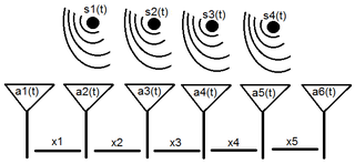
Array processing is a wide area of research in the field of signal processing that extends from the simplest form of 1 dimensional line arrays to 2 and 3 dimensional array geometries. Array structure can be defined as a set of sensors that are spatially separated, e.g. radio antenna and seismic arrays. The sensors used for a specific problem may vary widely, for example microphones, accelerometers and telescopes. However, many similarities exist, the most fundamental of which may be an assumption of wave propagation. Wave propagation means there is a systemic relationship between the signal received on spatially separated sensors. By creating a physical model of the wave propagation, or in machine learning applications a training data set, the relationships between the signals received on spatially separated sensors can be leveraged for many applications.

Machine olfaction is the automated simulation of the sense of smell. An emerging application in modern engineering, it involves the use of robots or other automated systems to analyze air-borne chemicals. Such an apparatus is often called an electronic nose or e-nose. The development of machine olfaction is complicated by the fact that e-nose devices to date have responded to a limited number of chemicals, whereas odors are produced by unique sets of odorant compounds. The technology, though still in the early stages of development, promises many applications, such as: quality control in food processing, detection and diagnosis in medicine, detection of drugs, explosives and other dangerous or illegal substances, disaster response, and environmental monitoring.

<span class="mw-page-title-main">Acoustic location</span> Use of reflected sound waves to locate objects

Acoustic location is a method of determining the position of an object or sound source by using sound waves. Location can take place in gases, liquids, and in solids.

In land warfare, artillery sound ranging is a method of determining the coordinates of a hostile battery using data derived from the sound of its guns firing, so called target acquisition.

Geophysical survey is the systematic collection of geophysical data for spatial studies. Detection and analysis of the geophysical signals forms the core of Geophysical signal processing. The magnetic and gravitational fields emanating from the Earth's interior hold essential information concerning seismic activities and the internal structure. Hence, detection and analysis of the electric and Magnetic fields is very crucial. As the Electromagnetic and gravitational waves are multi-dimensional signals, all the 1-D transformation techniques can be extended for the analysis of these signals as well. Hence this article also discusses multi-dimensional signal processing techniques.

Time-domain thermoreflectance is a method by which the thermal properties of a material can be measured, most importantly thermal conductivity. This method can be applied most notably to thin film materials, which have properties that vary greatly when compared to the same materials in bulk. The idea behind this technique is that once a material is heated up, the change in the reflectance of the surface can be utilized to derive the thermal properties. The reflectivity is measured with respect to time, and the data received can be matched to a model with coefficients that correspond to thermal properties.

An acoustic camera is an imaging device used to locate sound sources and to characterize them. It consists of a group of microphones, also called a microphone array, from which signals are simultaneously collected and processed to form a representation of the location of the sound sources.

Perceptual-based 3D sound localization is the application of knowledge of the human auditory system to develop 3D sound localization technology.

The spectral correlation density (SCD), sometimes also called the cyclic spectral density or spectral correlation function, is a function that describes the cross-spectral density of all pairs of frequency-shifted versions of a time-series. The spectral correlation density applies only to cyclostationary processes because stationary processes do not exhibit spectral correlation. Spectral correlation has been used both in signal detection and signal classification. The spectral correlation density is closely related to each of the bilinear time-frequency distributions, but is not considered one of Cohen's class of distributions.

Beamforming is a signal processing technique used to spatially select propagating waves. In order to implement beamforming on digital hardware the received signals need to be discretized. This introduces quantization error, perturbing the array pattern. For this reason, the sample rate must be generally much greater than the Nyquist rate.

Steered-response power (SRP) is a family of acoustic source localization algorithms that can be interpreted as a beamforming-based approach that searches for the candidate position or direction that maximizes the output of a steered delay-and-sum beamformer.

3D sound reconstruction is the application of reconstruction techniques to 3D sound localization technology. These methods of reconstructing three-dimensional sound are used to recreate sounds to match natural environments and provide spatial cues of the sound source. They also see applications in creating 3D visualizations on a sound field to include physical aspects of sound waves including direction, pressure, and intensity. This technology is used in entertainment to reproduce a live performance through computer speakers. The technology is also used in military applications to determine location of sound sources. Reconstructing sound fields is also applicable to medical imaging to measure points in ultrasound.

3D sound is most commonly defined as the daily human experience of sounds. The sounds arrive to the ears from every direction and varying distances, which contribute to the three-dimensional aural image humans hear. Scientists and engineers who work with 3D sound work to accurately synthesize the complexity of real-world sounds.

References

  1. Keyrouz, Fakheredine; Diepold, Klaus; Keyrouz, Shady (September 2007). "High performance 3D sound localization for surveillance applications". 2007 IEEE Conference on Advanced Video and Signal Based Surveillance. pp. 563–6. doi:10.1109/AVSS.2007.4425372. ISBN   978-1-4244-1695-0. S2CID   11238184.
  2. Kjær, Brüel. "Noise Source Identification". bksv.com. Brüel & Kjær.
  3. Goldstein, E.Bruce (2009-02-13). Sensation and Perception (Eighth ed.). Cengage Learning. pp. 293–297. ISBN   978-0-495-60149-4.
  4. Kjær, Brüel. "Listening in 3D". Brüel & Kjær.
  5. 1 2 Nakashima, H.; Mukai, T. (2005). "3D Sound Source Localization System Based on Learning of Binaural Hearing". 2005 IEEE International Conference on Systems, Man and Cybernetics. Vol. 4. pp. 3534–3539. doi:10.1109/ICSMC.2005.1571695. ISBN   0-7803-9298-1. S2CID   7446711.
  6. Liang, Yun; Cui, Zheng; Zhao, Shengkui; Rupnow, Kyle; Zhang, Yihao; Jones, Douglas L.; Chen, Deming (2012). "Real-time implementation and performance optimization of 3D sound localization on GPUs". Automation and Test in Europe Conference and Exhibition: 832–5. ISSN   1530-1591.
  7. Fernandez Comesana, D.; Steltenpool, S.; Korbasiewicz, M.; Tijs, E. (2015). "Direct acoustic vector field mapping: new scanning tools for measuring 3D sound intensity in 3D space". Proceedings of Euronoise: 891–895. ISSN   2226-5147.
  8. Ephraim, Y.; Malah, D. (Dec 1984). "Speech enhancement using a minimum-mean square error short-time spectral amplitude estimator". IEEE Transactions on Acoustics, Speech, and Signal Processing. 32 (6): 1109–21. doi:10.1109/TASSP.1984.1164453. ISSN   0096-3518.
  9. Valin, J.M.; Michaud, F.; Rouat, Jean (14–19 May 2006). "Robust 3D Localization and Tracking of Sound Sources Using Beamforming and Particle Filtering". 2006 IEEE International Conference on Acoustics Speech and Signal Processing Proceedings. Vol. 4. p. IV. arXiv: 1604.01642 . doi:10.1109/ICASSP.2006.1661100. ISBN   978-1-4244-0469-8. ISSN   1520-6149. S2CID   557491.
  10. Pérez Cabo, Daniel; de Bree, Hans Elias; Fernandez Comesaña, Daniel; Sobreira Seoane, Manuel. "Real life harmonic source localization using a network of acoustic vector sensors". EuroNoise 2015.
  11. Salas Natera, M.A.; Martinez Rodriguez-Osorio, R.; de Haro Ariet, L.; Sierra Perez, M. (2012). "Calibration Proposal for New Antenna Array Architectures and Technologies for Space Communications". IEEE Antennas and Wireless Propagation Letters. 11: 1129–32. Bibcode:2012IAWPL..11.1129S. doi:10.1109/LAWP.2012.2215952. ISSN   1536-1225.
  12. Ishi, C.T.; Even, J.; Hagita, N. (November 2013). "Using multiple microphone arrays and reflections for 3D localization of sound sources". 2013 IEEE/RSJ International Conference on Intelligent Robots and Systems. pp. 3937–42. doi:10.1109/IROS.2013.6696919. ISBN   978-1-4673-6358-7. S2CID   16043629.
  13. "Reducing noise emissions from Lontra's LP2 compressor".
  14. Keyrouz, Fakheredine; Diepold, Klaus (2006). "An Enhanced Binaural 3D Sound Localization Algorithm". 2006 IEEE International Symposium on Signal Processing and Information Technology. pp. 662–665. doi:10.1109/ISSPIT.2006.270883. ISBN   0-7803-9754-1. S2CID   14042947.
  15. Hyun-Don Kim; Komatani, K.; Ogata, T.; Okuno,H.G. (Jan 2008). Evaluation of Two-Channel-Based Sound Source Localization using 3D Moving Sound Creation Tool. ICERI 2008. doi:10.1109/ICKS.2008.25.
  16. Tabrikian,J.; Messer,H. (Jan 1996). "Three-Dimensional Source Localization in a Waveguide". IEEE Transactions on Signal Processing. 44 (1): 1–13. Bibcode:1996ITSP...44....1T. doi:10.1109/78.482007.
  17. Gala, Deepak; Lindsay, Nathan; Sun, Liang (July 2018). "Realtime Active Sound Source Localization for Unmanned Ground Robots Using a Self-Rotational Bi-Microphone Array". Journal of Intelligent & Robotic Systems. 95 (3): 935–954. arXiv: 1804.03372 . doi:10.1007/s10846-018-0908-3. S2CID   4745823.
  18. Gala, Deepak; Lindsay, Nathan; Sun, Liang (June 2018). Three-dimensional sound source localization for unmanned ground vehicles with a self-rotational two-microphone array. CDSR 2018. doi: 10.11159/cdsr18.104 .
  19. Gala, Deepak; Lindsay, Nathan; Sun, Liang (Oct 2021). Multi-Sound-Source Localization Using Machine Learning for Small Autonomous Unmanned Vehicles with a Self-Rotating Bi-Microphone Array. Journal of Intelligent & Robotic Systems. Vol. 103, no. 3. arXiv: 1804.05111 . doi:10.1007/s10846-021-01481-4.
  20. Keyrouz, Fakheredine; Diepold, Klaus (May 2008). "A novel biologically inspired neural network solution for robotic 3D sound source sensing". Soft Computing. 12 (7): 721–9. doi:10.1007/s00500-007-0249-9. ISSN   1432-7643. S2CID   30037380.
  21. Hill, P.A.; Nelson, P.A.; Kirkeby, O.; Hamada, H. (December 2000). "Resolution of front-back confusion in virtual acoustic imaging systems". Journal of the Acoustical Society of America. 108 (6): 2901–10. Bibcode:2000ASAJ..108.2901H. doi:10.1121/1.1323235. ISSN   0001-4966. PMID   11144583.
  22. Noriaki, Sakamoto; wataru, Kobayashi; Takao, Onoye; Isao, Shirakawa (2001). "DSP implementation of 3D sound localization algorithm for monaural sound source". ICECS 2001. 8th IEEE International Conference on Electronics, Circuits and Systems (Cat. No.01EX483). Vol. 2. pp. 1061–1064. doi:10.1109/ICECS.2001.957673. ISBN   978-0-7803-7057-9. S2CID   60528168.
  23. Saxena, A.; Ng, A.Y. (2009). "Learning sound location from a single microphone". 2009 IEEE International Conference on Robotics and Automation. pp. 1737–1742. doi:10.1109/ROBOT.2009.5152861. ISBN   978-1-4244-2788-8. S2CID   14665341.