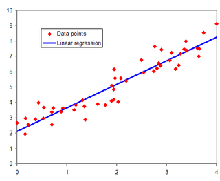
In statistics, the term linear model refers to any model which assumes linearity in the system. The most common occurrence is in connection with regression models and the term is often taken as synonymous with linear regression model. However, the term is also used in time series analysis with a different meaning. In each case, the designation "linear" is used to identify a subclass of models for which substantial reduction in the complexity of the related statistical theory is possible.
In statistics, the Gauss–Markov theorem states that the ordinary least squares (OLS) estimator has the lowest sampling variance within the class of linear unbiased estimators, if the errors in the linear regression model are uncorrelated, have equal variances and expectation value of zero. The errors do not need to be normal for the theorem to apply, nor do they need to be independent and identically distributed.

In statistical modeling, regression analysis is a set of statistical processes for estimating the relationships between a dependent variable and one or more independent variables. The most common form of regression analysis is linear regression, in which one finds the line that most closely fits the data according to a specific mathematical criterion. For example, the method of ordinary least squares computes the unique line that minimizes the sum of squared differences between the true data and that line. For specific mathematical reasons, this allows the researcher to estimate the conditional expectation of the dependent variable when the independent variables take on a given set of values. Less common forms of regression use slightly different procedures to estimate alternative location parameters or estimate the conditional expectation across a broader collection of non-linear models.
The general linear model or general multivariate regression model is a compact way of simultaneously writing several multiple linear regression models. In that sense it is not a separate statistical linear model. The various multiple linear regression models may be compactly written as
Functional data analysis (FDA) is a branch of statistics that analyses data providing information about curves, surfaces or anything else varying over a continuum. In its most general form, under an FDA framework, each sample element of functional data is considered to be a random function. The physical continuum over which these functions are defined is often time, but may also be spatial location, wavelength, probability, etc. Intrinsically, functional data are infinite dimensional. The high intrinsic dimensionality of these data brings challenges for theory as well as computation, where these challenges vary with how the functional data were sampled. However, the high or infinite dimensional structure of the data is a rich source of information and there are many interesting challenges for research and data analysis.
The partition of sums of squares is a concept that permeates much of inferential statistics and descriptive statistics. More properly, it is the partitioning of sums of squared deviations or errors. Mathematically, the sum of squared deviations is an unscaled, or unadjusted measure of dispersion. When scaled for the number of degrees of freedom, it estimates the variance, or spread of the observations about their mean value. Partitioning of the sum of squared deviations into various components allows the overall variability in a dataset to be ascribed to different types or sources of variability, with the relative importance of each being quantified by the size of each component of the overall sum of squares.
In statistics, a generalized additive model (GAM) is a generalized linear model in which the linear response variable depends linearly on unknown smooth functions of some predictor variables, and interest focuses on inference about these smooth functions.
Nonparametric regression is a category of regression analysis in which the predictor does not take a predetermined form but is constructed according to information derived from the data. That is, no parametric form is assumed for the relationship between predictors and dependent variable. Nonparametric regression requires larger sample sizes than regression based on parametric models because the data must supply the model structure as well as the model estimates.
In statistics, semiparametric regression includes regression models that combine parametric and nonparametric models. They are often used in situations where the fully nonparametric model may not perform well or when the researcher wants to use a parametric model but the functional form with respect to a subset of the regressors or the density of the errors is not known. Semiparametric regression models are a particular type of semiparametric modelling and, since semiparametric models contain a parametric component, they rely on parametric assumptions and may be misspecified and inconsistent, just like a fully parametric model.
Bootstrapping is any test or metric that uses random sampling with replacement, and falls under the broader class of resampling methods. Bootstrapping assigns measures of accuracy to sample estimates. This technique allows estimation of the sampling distribution of almost any statistic using random sampling methods.
Smoothing splines are function estimates, , obtained from a set of noisy observations of the target , in order to balance a measure of goodness of fit of to with a derivative based measure of the smoothness of . They provide a means for smoothing noisy data. The most familiar example is the cubic smoothing spline, but there are many other possibilities, including for the case where is a vector quantity.
In statistics, projection pursuit regression (PPR) is a statistical model developed by Jerome H. Friedman and Werner Stuetzle that extends additive models. This model adapts the additive models in that it first projects the data matrix of explanatory variables in the optimal direction before applying smoothing functions to these explanatory variables.
In statistics, the backfitting algorithm is a simple iterative procedure used to fit a generalized additive model. It was introduced in 1985 by Leo Breiman and Jerome Friedman along with generalized additive models. In most cases, the backfitting algorithm is equivalent to the Gauss–Seidel method, an algorithm used for solving a certain linear system of equations.
In statistics, the two-way analysis of variance (ANOVA) is an extension of the one-way ANOVA that examines the influence of two different categorical independent variables on one continuous dependent variable. The two-way ANOVA not only aims at assessing the main effect of each independent variable but also if there is any interaction between them.
In statistics and in machine learning, a linear predictor function is a linear function of a set of coefficients and explanatory variables, whose value is used to predict the outcome of a dependent variable. This sort of function usually comes in linear regression, where the coefficients are called regression coefficients. However, they also occur in various types of linear classifiers, as well as in various other models, such as principal component analysis and factor analysis. In many of these models, the coefficients are referred to as "weights".
In statistics, the class of vector generalized linear models (VGLMs) was proposed to enlarge the scope of models catered for by generalized linear models (GLMs). In particular, VGLMs allow for response variables outside the classical exponential family and for more than one parameter. Each parameter can be transformed by a link function. The VGLM framework is also large enough to naturally accommodate multiple responses; these are several independent responses each coming from a particular statistical distribution with possibly different parameter values.
Functional regression is a version of regression analysis when responses or covariates include functional data. Functional regression models can be classified into four types depending on whether the responses or covariates are functional or scalar: (i) scalar responses with functional covariates, (ii) functional responses with scalar covariates, (iii) functional responses with functional covariates, and (iv) scalar or functional responses with functional and scalar covariates. In addition, functional regression models can be linear, partially linear, or nonlinear. In particular, functional polynomial models, functional single and multiple index models and functional additive models are three special cases of functional nonlinear models.
In statistics, functional additive models (FAM) can be viewed as extensions of generalized functional linear models where the linearity assumption between the response and the functional linear predictor is replaced by an additivity assumption.
A partially linear model is a form of semiparametric model, since it contains parametric and nonparametric elements. Application of the least squares estimators is available to partially linear model, if the hypothesis of the known of nonparametric element is valid. Partially linear equations were first used in the analysis of the relationship between temperature and usage of electricity by Engle, Granger, Rice and Weiss (1986). Typical application of partially linear model in the field of Microeconomics is presented by Tripathi in the case of profitability of firm's production in 1997. Also, partially linear model applied successfully in some other academic field. In 1994, Zeger and Diggle introduced partially linear model into biometrics. In environmental science, Parda-Sanchez et al. used partially linear model to analysis collected data in 2000. So far, partially linear model was optimized in many other statistic methods. In 1988, Robinson applied Nadaraya-Waston kernel estimator to test the nonparametric element to build a least-squares estimator After that, in 1997, local linear method was found by Truong.
Nonlinear mixed-effects models constitute a class of statistical models generalizing linear mixed-effects models. Like linear mixed-effects models, they are particularly useful in settings where there are multiple measurements within the same statistical units or when there are dependencies between measurements on related statistical units. Nonlinear mixed-effects models are applied in many fields including medicine, public health, pharmacology, and ecology.


