Buffer analysis

Last updated November 22, 2023

In geographic information systems (GIS) and spatial analysis, buffer analysis is the determination of a zone around a geographic feature containing locations that are within a specified distance of that feature, the buffer zone (or just buffer).^[1] A buffer is likely the most commonly used tool within the proximity analysis methods.^[2]

History

The buffer operation has been a core part of GIS functionality since the original integrated GIS software packages of the late 1970s and early 1980s, such as ARC/INFO, Odyssey, and MOSS. Although it has been one of the most widely used GIS operations in subsequent years, in a wide variety of applications, there has been little published research on the tool itself, except for the occasional development of a more efficient algorithm.^[3]

Basic algorithm

The fundamental method to create a buffer around a geographic feature stored in a vector data model, with a given radius r is as follows:^[4]

Single point: Create a circle around the point with radius r.
Polyline, which consists of an ordered list of points (vertices) connected by straight lines. This is also used for the boundary of a polygon.

Create a circle buffer around each vertex
Create a rectangle along each line segment by creating a duplicate line segment offset the distance r perpendicular to each side.
Merge or dissolve the rectangles and circles into a single polygon.

Software implementations of the buffer operation typically use alterations of this strategy to process more efficiently and accurately.

In Mathematics, GIS Buffer operation is a Minkowski Sum (or difference) of a geometry and a disk. Other terms used: Offsetting a Polygon^[5].

Planar vs. geodesic distance

Traditional implementations assumed the buffer was being created on a planar cartesian coordinate space (i.e., created by a map projection) using Euclidean geometry, because the mathematics and computation involved is relatively simple, which was important given the computing power available in the late 1970s. Due to the inherent distortions caused by map projections, the buffer computed this way will not be identical to one drawn on the surface of the Earth; at a local scale, the difference is negligible, but at larger scales, the error can be significant.

Some current software, such as Esri ArcGIS Pro, offer the option to compute buffers using geodesic distance, using a similar algorithm but calculated using spherical trigonometry, including representing the lines between vertices as great circles.^[4] Other implementations use a workaround by first reprojecting the feature to a projection that minimizes distortion in that location, then computing the planar buffer.^[6]

Options

GIS software may offer variations on the basic algorithm, which may be useful in different applications:^[1]

Endcaps at the end of linear buffers are rounded by default, but may be squared off or a butt end (truncated at the final vertex).
Side preference may be important, such as needing the buffer on only one side of a line, or on a polygon, selecting only the outer buffer or the inner buffer (sometimes called a setback).
Variable width, in which the features in a layer may be buffered using different radii, usually given by an attribute.
Common buffers, in which the buffers for each feature in a layer are dissolved into a single polygon. This is most commonly used when one is not concerned about which feature is near each point in space, only that a point is nearby some (anonymous) feature.

External links

OGC ST_Buffer function (PostGIS implementation)
buffer function in turfjs
BufferOp in JTS, the library at the foundation of many open-source GIS implementations
v.buffer command in GRASS
Buffer (Analysis) tool in Esri ArcGIS Pro

Related Research Articles

<span class="mw-page-title-main">Geometric primitive</span> Basic shapes represented in vector graphics

In vector computer graphics, CAD systems, and geographic information systems, geometric primitive is the simplest geometric shape that the system can handle. Sometimes the subroutines that draw the corresponding objects are called "geometric primitives" as well. The most "primitive" primitives are point and straight line segment, which were all that early vector graphics systems had.

<span class="mw-page-title-main">Graph drawing</span> Visualization of node-link graphs

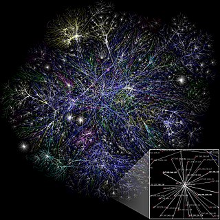
Graph drawing is an area of mathematics and computer science combining methods from geometric graph theory and information visualization to derive two-dimensional depictions of graphs arising from applications such as social network analysis, cartography, linguistics, and bioinformatics.

The point location problem is a fundamental topic of computational geometry. It finds applications in areas that deal with processing geometrical data: computer graphics, geographic information systems (GIS), motion planning, and computer aided design (CAD).

A transport network, or transportation network, is a network or graph in geographic space, describing an infrastructure that permits and constrains movement or flow. Examples include but are not limited to road networks, railways, air routes, pipelines, aqueducts, and power lines. The digital representation of these networks, and the methods for their analysis, is a core part of spatial analysis, geographic information systems, public utilities, and transport engineering. Network analysis is an application of the theories and algorithms of graph theory and is a form of proximity analysis.

Spatial network analysis software packages are analytic software used to prepare graph-based analysis of spatial networks. They stem from research fields in transportation, architecture, and urban planning. The earliest examples of such software include the work of Garrison (1962), Kansky (1963), Levin (1964), Harary (1969), Rittel (1967), Tabor (1970) and others in the 1960s and 70s. Specific packages address their domain-specific needs, including TransCAD for transportation, GIS for planning and geography, and Axman for Space syntax researchers.

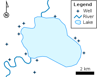
The shapefile format is a geospatial vector data format for geographic information system (GIS) software. It is developed and regulated by Esri as a mostly open specification for data interoperability among Esri and other GIS software products. The shapefile format can spatially describe vector features: points, lines, and polygons, representing, for example, water wells, rivers, and lakes. Each item usually has attributes that describe it, such as name or temperature.

ArcGIS is a family of client, server and online geographic information system (GIS) software developed and maintained by Esri.

gvSIG, geographic information system (GIS), is a desktop application designed for capturing, storing, handling, analyzing and deploying any kind of referenced geographic information in order to solve complex management and planning problems. gvSIG is known for having a user-friendly interface, being able to access the most common formats, both vector and raster ones. It features a wide range of tools for working with geographic-like information.

A spatial database is a general-purpose database that has been enhanced to include spatial data that represents objects defined in a geometric space, along with tools for querying and analyzing such data.

JTS Topology Suite is an open-source Java software library that provides an object model for Euclidean planar linear geometry together with a set of fundamental geometric functions. JTS is primarily intended to be used as a core component of vector-based geomatics software such as geographical information systems. It can also be used as a general-purpose library providing algorithms in computational geometry.

<span class="mw-page-title-main">Straight skeleton</span> Method in geometry for representing a polygon by a topological skeleton

In geometry, a straight skeleton is a method of representing a polygon by a topological skeleton. It is similar in some ways to the medial axis but differs in that the skeleton is composed of straight line segments, while the medial axis of a polygon may involve parabolic curves. However, both are homotopy-equivalent to the underlying polygon.

Map algebra is an algebra for manipulating geographic data, primarily fields. Developed by Dr. Dana Tomlin and others in the late 1970s, it is a set of primitive operations in a geographic information system (GIS) which allows one or more raster layers ("maps") of similar dimensions to produce a new raster layer (map) using mathematical or other operations such as addition, subtraction etc.

Algorithms that construct convex hulls of various objects have a broad range of applications in mathematics and computer science.

A geographic data model, geospatial data model, or simply data model in the context of geographic information systems, is a mathematical and digital structure for representing phenomena over the Earth. Generally, such data models represent various aspects of these phenomena by means of geographic data, including spatial locations, attributes, change over time, and identity. For example, the vector data model represents geography as collections of points, lines, and polygons, and the raster data model represent geography as cell matrices that store numeric values. Data models are implemented throughout the GIS ecosystem, including the software tools for data management and spatial analysis, data stored in a variety of GIS file formats, specifications and standards, and specific designs for GIS installations.

Proximity analysis is a class of spatial analysis tools and algorithms that employ geographic distance as a central principle. Distance is fundamental to geographic inquiry and spatial analysis, due to principles such as the friction of distance, Tobler's first law of geography, and Spatial autocorrelation, which are incorporated into analytical tools. Proximity methods are thus used in a variety of applications, especially those that involve movement and interaction.

Layered graph drawing or hierarchical graph drawing is a type of graph drawing in which the vertices of a directed graph are drawn in horizontal rows or layers with the edges generally directed downwards. It is also known as Sugiyama-style graph drawing after Kozo Sugiyama, who first developed this drawing style.

<span class="mw-page-title-main">Geospatial topology</span> Type of spatial relationship

Geospatial topology is the study and application of qualitative spatial relationships between geographic features, or between representations of such features in geographic information, such as in geographic information systems (GIS). For example, the fact that two regions overlap or that one contains the other are examples of topological relationships. It is thus the application of the mathematics of topology to GIS, and is distinct from, but complementary to the many aspects of geographic information that are based on quantitative spatial measurements through coordinate geometry. Topology appears in many aspects of geographic information science and GIS practice, including the discovery of inherent relationships through spatial query, vector overlay and map algebra; the enforcement of expected relationships as validation rules stored in geospatial data; and the use of stored topological relationships in applications such as network analysis. Spatial topology is the generalization of geospatial topology for non-geographic domains, e.g., CAD software.

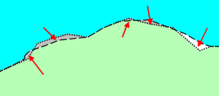
A sliver polygon, in the context of Geographic Information Systems (GIS), is a small polygon found in vector data that is an artifact of error rather than representing a real-world feature. They have been a recognized source of error since overlay was first invented in the 1970s.

This is a glossary of terms relating to computer graphics.

Vector overlay is an operation in a geographic information system (GIS) for integrating two or more vector spatial data sets. Terms such as polygon overlay, map overlay, and topological overlay are often used synonymously, although they are not identical in the range of operations they include. Overlay has been one of the core elements of spatial analysis in GIS since its early development. Some overlay operations, especially Intersect and Union, are implemented in all GIS software and are used in a wide variety of analytical applications, while others are less common.

References

1 2 de Smith, Michael J.; Goodchild, Michael F.; Longley, Paul A. (2018). "4.4.5 Buffering". Geospatial Analysis: A Comprehensive Guide to Principles, Techniques, and Software Tools (6th ed.).
↑ Wade, T. and Smmer, S. eds. A to Z GIS
↑ Bhatia, Sumeet; Vira, Viral; Choksi, Deepak; Venkatachalam, P. (2012). "An algorithm for generating geometric buffers for vector feature layers". Geo-spatial Information Science. 16 (2): 130–138. doi: 10.1080/10095020.2012.747643 .
1 2 "How Buffer (Analysis) Works". ArcGIS Pro Documentation. Esri. Retrieved 16 March 2021.
↑ "CGAL 5.6 - 2D Minkowski Sums: User Manual". doc.cgal.org. Retrieved 2023-11-21.
↑ "ST_Buffer". PostGIS documentation. Archived from the original on 2021-05-07. Retrieved 2012-11-02.

This technology-related article is a stub. You can help Wikipedia by expanding it.

This page is based on this Wikipedia article
Text is available under the CC BY-SA 4.0 license; additional terms may apply.
Images, videos and audio are available under their respective licenses.

[desmith-1] 1 2 de Smith, Michael J.; Goodchild, Michael F.; Longley, Paul A. (2018). "4.4.5 Buffering". Geospatial Analysis: A Comprehensive Guide to Principles, Techniques, and Software Tools (6th ed.).

[2] Wade, T. and Smmer, S. eds. A to Z GIS

[bhatia-3] Bhatia, Sumeet; Vira, Viral; Choksi, Deepak; Venkatachalam, P. (2012). "An algorithm for generating geometric buffers for vector feature layers". Geo-spatial Information Science. 16 (2): 130–138. doi: 10.1080/10095020.2012.747643 .

[arcgis-4] 1 2 "How Buffer (Analysis) Works". ArcGIS Pro Documentation. Esri. Retrieved 16 March 2021.

[5] "CGAL 5.6 - 2D Minkowski Sums: User Manual". doc.cgal.org. Retrieved 2023-11-21.

[postgis-6] "ST_Buffer". PostGIS documentation. Archived from the original on 2021-05-07. Retrieved 2012-11-02.

[1]

[2]

[3]

[4]

[5]

[6]