

Common spatial pattern (CSP) is a mathematical procedure used in signal processing for separating a multivariate signal into additive subcomponents which have maximum differences in variance between two windows. [1]
Common spatial pattern (CSP) is a mathematical procedure used in signal processing for separating a multivariate signal into additive subcomponents which have maximum differences in variance between two windows. [1]
Let of size and of size be two windows of a multivariate signal, where is the number of signals and and are the respective number of samples.
The CSP algorithm determines the component such that the ratio of variance (or second-order moment) is maximized between the two windows:
The solution is given by computing the two covariance matrices:
Then, the simultaneous diagonalization of those two matrices (also called generalized eigenvalue decomposition) is realized. We find the matrix of eigenvectors and the diagonal matrix of eigenvalues sorted by decreasing order such that:
and
with the identity matrix.
This is equivalent to the eigendecomposition of :
The eigenvectors composing are components with variance ratio between the two windows equal to their corresponding eigenvalue:
The vectorial subspace generated by the first eigenvectors will be the subspace maximizing the variance ratio of all components belonging to it:
On the same way, the vectorial subspace generated by the last eigenvectors will be the subspace minimizing the variance ratio of all components belonging to it:
CSP can be applied after a mean subtraction (a.k.a. "mean centering") on signals in order to realize a variance ratio optimization. Otherwise CSP optimizes the ratio of second-order moment.
Linear discriminant analysis (LDA) and CSP apply in different circumstances. LDA separates data that have different means, by finding a rotation that maximizes the (normalized) distance between the centers of the two sets of data. On the other hand, CSP ignores the means. Thus CSP is good, for example, in separating the signal from the noise in an event-related potential (ERP) experiment because both distributions have zero mean and there is no distinction for LDA to separate. Thus CSP finds a projection that makes the variance of the components of the average ERP as large as possible so the signal stands out above the noise.
The CSP method can be applied to multivariate signals in generally, is commonly found in application to electroencephalographic (EEG) signals. Particularly, the method is often used in brain–computer interfaces to retrieve the component signals which best transduce the cerebral activity for a specific task (e.g. hand movement). [4] It can also be used to separate artifacts from EEG signals. [2]
CSP can be adapted for the analysis of the event-related potentials. [5]

In mathematics, the discrete Fourier transform (DFT) converts a finite sequence of equally-spaced samples of a function into a same-length sequence of equally-spaced samples of the discrete-time Fourier transform (DTFT), which is a complex-valued function of frequency. The interval at which the DTFT is sampled is the reciprocal of the duration of the input sequence. An inverse DFT is a Fourier series, using the DTFT samples as coefficients of complex sinusoids at the corresponding DTFT frequencies. It has the same sample-values as the original input sequence. The DFT is therefore said to be a frequency domain representation of the original input sequence. If the original sequence spans all the non-zero values of a function, its DTFT is continuous, and the DFT provides discrete samples of one cycle. If the original sequence is one cycle of a periodic function, the DFT provides all the non-zero values of one DTFT cycle.
The weighted arithmetic mean is similar to an ordinary arithmetic mean, except that instead of each of the data points contributing equally to the final average, some data points contribute more than others. The notion of weighted mean plays a role in descriptive statistics and also occurs in a more general form in several other areas of mathematics.

In probability theory and statistics, the multivariate normal distribution, multivariate Gaussian distribution, or joint normal distribution is a generalization of the one-dimensional (univariate) normal distribution to higher dimensions. One definition is that a random vector is said to be k-variate normally distributed if every linear combination of its k components has a univariate normal distribution. Its importance derives mainly from the multivariate central limit theorem. The multivariate normal distribution is often used to describe, at least approximately, any set of (possibly) correlated real-valued random variables each of which clusters around a mean value.

The principal components of a collection of points in a real p-space are a sequence of direction vectors, where the vector is the direction of a line that best fits the data while being orthogonal to the first vectors. Here, a best-fitting line is defined as one that minimizes the average squared distance from the points to the line. These directions constitute an orthonormal basis in which different individual dimensions of the data are linearly uncorrelated. Principal component analysis (PCA) is the process of computing the principal components and using them to perform a change of basis on the data, sometimes using only the first few principal components and ignoring the rest.
Ray transfer matrix analysis is a mathematical form for performing ray tracing calculations in sufficiently simple problems which can be solved considering only paraxial rays. Each optical element is described by a 2×2 ray transfer matrix which operates on a vector describing an incoming light ray to calculate the outgoing ray. Multiplication of the successive matrices thus yields a concise ray transfer matrix describing the entire optical system. The same mathematics is also used in accelerator physics to track particles through the magnet installations of a particle accelerator, see electron optics.
In mechanics and geometry, the 3D rotation group, often denoted SO(3), is the group of all rotations about the origin of three-dimensional Euclidean space under the operation of composition. By definition, a rotation about the origin is a transformation that preserves the origin, Euclidean distance, and orientation. Every non-trivial rotation is determined by its axis of rotation and its angle of rotation. Composing two rotations results in another rotation; every rotation has a unique inverse rotation; and the identity map satisfies the definition of a rotation. Owing to the above properties, the set of all rotations is a group under composition. Rotations are not commutative, making it a nonabelian group. Moreover, the rotation group has a natural structure as a manifold for which the group operations are smoothly differentiable; so it is in fact a Lie group. It is compact and has dimension 3.

In fluid dynamics, the Euler equations are a set of quasilinear hyperbolic equations governing adiabatic and inviscid flow. They are named after Leonhard Euler. The equations represent Cauchy equations of conservation of mass (continuity), and balance of momentum and energy, and can be seen as particular Navier–Stokes equations with zero viscosity and zero thermal conductivity. In fact, Euler equations can be obtained by linearization of some more precise continuity equations like Navier–Stokes equations in a local equilibrium state given by a Maxwellian. The Euler equations can be applied to incompressible and to compressible flow – assuming the flow velocity is a solenoidal field, or using another appropriate energy equation respectively. Historically, only the incompressible equations have been derived by Euler. However, fluid dynamics literature often refers to the full set – including the energy equation – of the more general compressible equations together as "the Euler equations".
In mathematics, the Heisenberg group, named after Werner Heisenberg, is the group of 3×3 upper triangular matrices of the form
In linear algebra, a rotation matrix is a transformation matrix that is used to perform a rotation in Euclidean space. For example, using the convention below, the matrix

In geometry, Euler's rotation theorem states that, in three-dimensional space, any displacement of a rigid body such that a point on the rigid body remains fixed, is equivalent to a single rotation about some axis that runs through the fixed point. It also means that the composition of two rotations is also a rotation. Therefore the set of rotations has a group structure, known as a rotation group.
In linear algebra, given a vector space V with a basis B of vectors indexed by an index set I, the dual set of B is a set B∗ of vectors in the dual space V∗ with the same index set I such that B and B∗ form a biorthogonal system. The dual set is always linearly independent but does not necessarily span V∗. If it does span V∗, then B∗ is called the dual basis or reciprocal basis for the basis B.
Estimation theory is a branch of statistics that deals with estimating the values of parameters based on measured empirical data that has a random component. The parameters describe an underlying physical setting in such a way that their value affects the distribution of the measured data. An estimator attempts to approximate the unknown parameters using the measurements.
FastICA is an efficient and popular algorithm for independent component analysis invented by Aapo Hyvärinen at Helsinki University of Technology. Like most ICA algorithms, FastICA seeks an orthogonal rotation of prewhitened data, through a fixed-point iteration scheme, that maximizes a measure of non-Gaussianity of the rotated components. Non-gaussianity serves as a proxy for statistical independence, which is a very strong condition and requires infinite data to verify. FastICA can also be alternatively derived as an approximative Newton iteration.

In applied mathematics, in particular the context of nonlinear system analysis, a phase plane is a visual display of certain characteristics of certain kinds of differential equations; a coordinate plane with axes being the values of the two state variables, say, or etc.. It is a two-dimensional case of the general n-dimensional phase space.
In linear algebra, an eigenvector or characteristic vector of a linear transformation is a nonzero vector that changes by a scalar factor when that linear transformation is applied to it. The corresponding eigenvalue, often denoted by , is the factor by which the eigenvector is scaled.
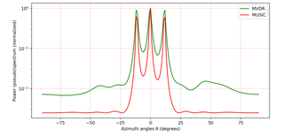
MUSIC is an algorithm used for frequency estimation and radio direction finding.
In statistical signal processing, the goal of spectral density estimation (SDE) is to estimate the spectral density of a random signal from a sequence of time samples of the signal. Intuitively speaking, the spectral density characterizes the frequency content of the signal. One purpose of estimating the spectral density is to detect any periodicities in the data, by observing peaks at the frequencies corresponding to these periodicities.
In linear algebra, eigendecomposition or sometimes spectral decomposition is the factorization of a matrix into a canonical form, whereby the matrix is represented in terms of its eigenvalues and eigenvectors. Only diagonalizable matrices can be factorized in this way.

In statistics, principal component regression (PCR) is a regression analysis technique that is based on principal component analysis (PCA). More specifically, PCR is used for estimating the unknown regression coefficients in a standard linear regression model.
A differential equation is a mathematical equation for an unknown function of one or several variables that relates the values of the function itself and of its derivatives of various orders. A matrix differential equation contains more than one function stacked into vector form with a matrix relating the functions to their derivatives.


