In probability theory, the expected value is a generalization of the weighted average. Informally, the expected value is the arithmetic mean of a large number of independently selected outcomes of a random variable.

In probability theory and statistics, variance is the expectation of the squared deviation of a random variable from its population mean or sample mean. Variance is a measure of dispersion, meaning it is a measure of how far a set of numbers is spread out from their average value. Variance has a central role in statistics, where some ideas that use it include descriptive statistics, statistical inference, hypothesis testing, goodness of fit, and Monte Carlo sampling. Variance is an important tool in the sciences, where statistical analysis of data is common. The variance is the square of the standard deviation, the second central moment of a distribution, and the covariance of the random variable with itself, and it is often represented by , , , , or .

In probability, and statistics, a multivariate random variable or random vector is a list of mathematical variables each of whose value is unknown, either because the value has not yet occurred or because there is imperfect knowledge of its value. The individual variables in a random vector are grouped together because they are all part of a single mathematical system — often they represent different properties of an individual statistical unit. For example, while a given person has a specific age, height and weight, the representation of these features of an unspecified person from within a group would be a random vector. Normally each element of a random vector is a real number.

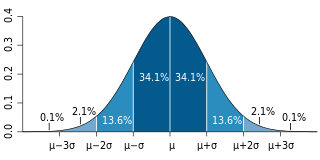
In probability theory and statistics, the multivariate normal distribution, multivariate Gaussian distribution, or joint normal distribution is a generalization of the one-dimensional (univariate) normal distribution to higher dimensions. One definition is that a random vector is said to be k-variate normally distributed if every linear combination of its k components has a univariate normal distribution. Its importance derives mainly from the multivariate central limit theorem. The multivariate normal distribution is often used to describe, at least approximately, any set of (possibly) correlated real-valued random variables each of which clusters around a mean value.

A Markov chain or Markov process is a stochastic model describing a sequence of possible events in which the probability of each event depends only on the state attained in the previous event. Informally, this may be thought of as, "What happens next depends only on the state of affairs now." A countably infinite sequence, in which the chain moves state at discrete time steps, gives a discrete-time Markov chain (DTMC). A continuous-time process is called a continuous-time Markov chain (CTMC). It is named after the Russian mathematician Andrey Markov.
A hidden Markov model (HMM) is a statistical Markov model in which the system being modeled is assumed to be a Markov process — call it — with unobservable ("hidden") states. As part of the definition, HMM requires that there be an observable process whose outcomes are "influenced" by the outcomes of in a known way. Since cannot be observed directly, the goal is to learn about by observing HMM has an additional requirement that the outcome of at time must be "influenced" exclusively by the outcome of at and that the outcomes of and at must not affect the outcome of at
A Bayesian network is a probabilistic graphical model that represents a set of variables and their conditional dependencies via a directed acyclic graph (DAG). Bayesian networks are ideal for taking an event that occurred and predicting the likelihood that any one of several possible known causes was the contributing factor. For example, a Bayesian network could represent the probabilistic relationships between diseases and symptoms. Given symptoms, the network can be used to compute the probabilities of the presence of various diseases.
In mathematics, a stochastic matrix is a square matrix used to describe the transitions of a Markov chain. Each of its entries is a nonnegative real number representing a probability. It is also called a probability matrix, transition matrix, substitution matrix, or Markov matrix. The stochastic matrix was first developed by Andrey Markov at the beginning of the 20th century, and has found use throughout a wide variety of scientific fields, including probability theory, statistics, mathematical finance and linear algebra, as well as computer science and population genetics. There are several different definitions and types of stochastic matrices:

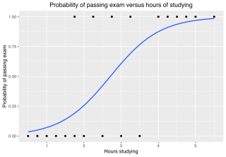
In statistics, the logistic model is a statistical model that models the probability of an event taking place by having the log-odds for the event be a linear combination of one or more independent variables. In regression analysis, logistic regression is estimating the parameters of a logistic model. Formally, in binary logistic regression there is a single binary dependent variable, coded by an indicator variable, where the two values are labeled "0" and "1", while the independent variables can each be a binary variable or a continuous variable. The corresponding probability of the value labeled "1" can vary between 0 and 1, hence the labeling; the function that converts log-odds to probability is the logistic function, hence the name. The unit of measurement for the log-odds scale is called a logit, from logistic unit, hence the alternative names. See § Background and § Definition for formal mathematics, and § Example for a worked example.
Pearson's chi-squared test is a statistical test applied to sets of categorical data to evaluate how likely it is that any observed difference between the sets arose by chance. It is the most widely used of many chi-squared tests – statistical procedures whose results are evaluated by reference to the chi-squared distribution. Its properties were first investigated by Karl Pearson in 1900. In contexts where it is important to improve a distinction between the test statistic and its distribution, names similar to Pearson χ-squared test or statistic are used.
In probability theory and statistics, the marginal distribution of a subset of a collection of random variables is the probability distribution of the variables contained in the subset. It gives the probabilities of various values of the variables in the subset without reference to the values of the other variables. This contrasts with a conditional distribution, which gives the probabilities contingent upon the values of the other variables.
In statistics, Gibbs sampling or a Gibbs sampler is a Markov chain Monte Carlo (MCMC) algorithm for obtaining a sequence of observations which are approximated from a specified multivariate probability distribution, when direct sampling is difficult. This sequence can be used to approximate the joint distribution ; to approximate the marginal distribution of one of the variables, or some subset of the variables ; or to compute an integral. Typically, some of the variables correspond to observations whose values are known, and hence do not need to be sampled.
The information bottleneck method is a technique in information theory introduced by Naftali Tishby, Fernando C. Pereira, and William Bialek. It is designed for finding the best tradeoff between accuracy and complexity (compression) when summarizing a random variable X, given a joint probability distribution p(X,Y) between X and an observed relevant variable Y - and self-described as providing "a surprisingly rich framework for discussing a variety of problems in signal processing and learning".
The general linear model or general multivariate regression model is a compact way of simultaneously writing several multiple linear regression models. In that sense it is not a separate statistical linear model. The various multiple linear regression models may be compactly written as

Given two random variables that are defined on the same probability space, the joint probability distribution is the corresponding probability distribution on all possible pairs of outputs. The joint distribution can just as well be considered for any given number of random variables. The joint distribution encodes the marginal distributions, i.e. the distributions of each of the individual random variables. It also encodes the conditional probability distributions, which deal with how the outputs of one random variable are distributed when given information on the outputs of the other random variable(s).
In statistics, ordinary least squares (OLS) is a type of linear least squares method for choosing the unknown parameters in a linear regression model by the principle of least squares: minimizing the sum of the squares of the differences between the observed dependent variable in the input dataset and the output of the (linear) function of the independent variable.
In probability theory and statistics, the Dirichlet-multinomial distribution is a family of discrete multivariate probability distributions on a finite support of non-negative integers. It is also called the Dirichlet compound multinomial distribution (DCM) or multivariate Pólya distribution. It is a compound probability distribution, where a probability vector p is drawn from a Dirichlet distribution with parameter vector , and an observation drawn from a multinomial distribution with probability vector p and number of trials n. The Dirichlet parameter vector captures the prior belief about the situation and can be seen as a pseudocount: observations of each outcome that occur before the actual data is collected. The compounding corresponds to a Pólya urn scheme. It is frequently encountered in Bayesian statistics, machine learning, empirical Bayes methods and classical statistics as an overdispersed multinomial distribution.
The iterative proportional fitting procedure is the operation of finding the fitted matrix which is the closest to an initial matrix but with the row and column totals of a target matrix . The fitted matrix being of the form , where and are diagonal matrices such that has the margins of . Some algorithms can be chosen to perform biproportion. We have also the entropy maximization, information loss minimization or RAS which consists of factoring the matrix rows to match the specified row totals, then factoring its columns to match the specified column totals; each step usually disturbs the previous step’s match, so these steps are repeated in cycles, re-adjusting the rows and columns in turn, until all specified marginal totals are satisfactorily approximated. However, all algorithms give the same solution. In three- or more-dimensional cases, adjustment steps are applied for the marginals of each dimension in turn, the steps likewise repeated in cycles.

In probability theory, conditional probability is a measure of the probability of an event occurring, given that another event has already occurred. This particular method relies on event B occurring with some sort of relationship with another event A. In this event, the event B can be analyzed by a conditional probability with respect to A. If the event of interest is A and the event B is known or assumed to have occurred, "the conditional probability of A given B", or "the probability of A under the condition B", is usually written as P(A|B) or occasionally PB(A). This can also be understood as the fraction of probability B that intersects with A: .
In statistics, the class of vector generalized linear models (VGLMs) was proposed to enlarge the scope of models catered for by generalized linear models (GLMs). In particular, VGLMs allow for response variables outside the classical exponential family and for more than one parameter. Each parameter can be transformed by a link function. The VGLM framework is also large enough to naturally accommodate multiple responses; these are several independent responses each coming from a particular statistical distribution with possibly different parameter values.


