Cyclomatic complexity

Cyclomatic complexity is a software metric used to indicate the complexity of a program. It is a quantitative measure of the number of linearly independent paths through a program's source code. It was developed by Thomas J. McCabe, Sr. in 1976.

Cyclomatic complexity is computed using the control-flow graph of the program: the nodes of the graph correspond to indivisible groups of commands of a program, and a directed edge connects two nodes if the second command might be executed immediately after the first command. Cyclomatic complexity may also be applied to individual functions, modules, methods or classes within a program.

One testing strategy, called basis path testing by McCabe who first proposed it, is to test each linearly independent path through the program; in this case, the number of test cases will equal the cyclomatic complexity of the program. ^[1]

Description

Definition

A control-flow graph of a simple program. The program begins executing at the red node, then enters a loop (group of three nodes immediately below the red node). Exiting the loop, there is a conditional statement (group below the loop) and the program exits at the blue node. This graph has nine edges, eight nodes and one connected component, so the program's cyclomatic complexity is 9 − 8 + 2×1 = 3.

There are a number of ways to define cyclomatic complexity of a section of source code. One common way is the number of linearly independent paths within it; a set ${\displaystyle S}$ of paths is linearly independent if the edge set of any path ${\displaystyle P}$ in ${\displaystyle S}$ is not the union of edge sets of the paths in some subset of ${\displaystyle S/P}$. If the source code contained no control flow statements (conditionals or decision points) the complexity would be 1, since there would be only a single path through the code. If the code had one single-condition IF statement, there would be two paths through the code: one where the IF statement is TRUE and another one where it is FALSE, so the complexity would be 2. Two nested single-condition IFs, or one IF with two conditions, would produce a complexity of 3.

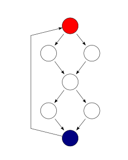
Another way to define the cyclomatic complexity of a program is to look at the control-flow graph of the program, a directed graph containing the basic blocks of the program, with an edge between two basic blocks if control may pass from the first to the second. The complexity M is then defined as ^[2]

$${\displaystyle M=E-N+2P,}$$

where

• E = the number of edges of the graph.
• N = the number of nodes of the graph.
• P = the number of connected components.

The same function, represented using the alternative formulation where each exit point is connected back to the entry point. This graph has 10 edges, eight nodes and one connected component, which also results in a cyclomatic complexity of 3 using the alternative formulation (10 − 8 + 1 = 3).

An alternative formulation of this is to use a graph in which each exit point is connected back to the entry point. In this case, the graph is strongly connected; the cyclomatic complexity of the program is equal to the cyclomatic number of its graph (also known as the first Betti number), which is defined as ^[2]

$${\displaystyle M=E-N+P.}$$

This may be seen as calculating the number of linearly independent cycles that exist in the graph: those cycles that do not contain other cycles within themselves. Because each exit point loops back to the entry point, there is at least one such cycle for each exit point.

For a single program (or subroutine or method), P is always equal to 1; a simpler formula for a single subroutine is ^[3]

$${\displaystyle M=E-N+2.}$$

Cyclomatic complexity may be applied to several such programs or subprograms at the same time (to all of the methods in a class, for example), and in these cases P will be equal to the number of programs in question; each subprogram will appear as a disconnected subset of the graph.

McCabe showed that the cyclomatic complexity of a structured program with only one entry point and one exit point is equal to the number of decision points ("if" statements or conditional loops) contained in that program plus one. This is true only for decision points counted at the lowest, machine-level instructions. ^[4] Decisions involving compound predicates like those found in high-level languages like IF cond1 AND cond2 THEN ... should be counted in terms of predicate variables involved; in this example, one should count two decision points because at machine level it is equivalent to IF cond1 THEN IF cond2 THEN .... ^{[2] [5]}

Cyclomatic complexity may be extended to a program with multiple exit points; in this case, it is equal to

$${\displaystyle \pi -s+2,}$$

where ${\displaystyle \pi }$ is the number of decision points in the program and s is the number of exit points. ^{[5] [6]}

Algebraic topology

An even subgraph of a graph (also known as an Eulerian subgraph) is one where every vertex is incident with an even number of edges; such subgraphs are unions of cycles and isolated vertices. Subgraphs will be identified with their edge sets, which is equivalent to only considering those even subgraphs which contain all vertices of the full graph.

The set of all even subgraphs of a graph is closed under symmetric difference, and may thus be viewed as a vector space over GF(2); this vector space is called the cycle space of the graph. The cyclomatic number of the graph is defined as the dimension of this space. Since GF(2) has two elements and the cycle space is necessarily finite, the cyclomatic number is also equal to the 2-logarithm of the number of elements in the cycle space.

A basis for the cycle space is easily constructed by first fixing a spanning forest of the graph, and then considering the cycles formed by one edge not in the forest and the path in the forest connecting the endpoints of that edge; these cycles form a basis for the cycle space. The cyclomatic number also equals the number of edges not in a maximal spanning forest of a graph. Since the number of edges in a maximal spanning forest of a graph is equal to the number of vertices minus the number of components, the formula ${\displaystyle E-N+P}$ for the cyclomatic number follows. ^[7]

Cyclomatic complexity can also be defined as a relative Betti number, the size of a relative homology group:

$${\displaystyle M:=b_{1}(G,t):=\operatorname {rank} H_{1}(G,t),}$$

which is read as "the rank of the first homology group of the graph G relative to the terminal nodes t". This is a technical way of saying "the number of linearly independent paths through the flow graph from an entry to an exit", where:

• "linearly independent" corresponds to homology; backtracking is not double-counted
• "paths" corresponds to first homology; a path is a one-dimensional object
• "relative" means the path must begin and end at an entry (or exit) point.

This cyclomatic complexity can be calculated. It may also be computed via absolute Betti number by identifying the terminal nodes on a given component, or drawing paths connecting the exits to the entrance. The new, augmented graph ${\displaystyle {\tilde {G}}}$ obtains

$${\displaystyle M=b_{1}({\tilde {G}})=\operatorname {rank} H_{1}({\tilde {G}}).}$$

It can also be computed via homotopy. If a (connected) control-flow graph is considered a one-dimensional CW complex called ${\displaystyle X}$, the fundamental group of ${\displaystyle X}$ will be ${\displaystyle \pi _{1}(X)\cong \mathbb {Z} ^{*n}}$. The value of ${\displaystyle n+1}$ is the cyclomatic complexity. The fundamental group counts how many loops there are through the graph up to homotopy, aligning as expected.

Interpretation

In his presentation "Software Quality Metrics to Identify Risk" ^[8] for the Department of Homeland Security, Tom McCabe introduces the following categorisation of cyclomatic complexity:

• 1 - 10: Simple procedure, little risk
• 11 - 20: More complex, moderate risk
• 21 - 50: Complex, high risk
• > 50: Untestable code, very high risk

Applications

Limiting complexity during development

One of McCabe's original applications was to limit the complexity of routines during program development; he recommended that programmers should count the complexity of the modules they are developing, and split them into smaller modules whenever the cyclomatic complexity of the module exceeded 10. ^[2] This practice was adopted by the NIST Structured Testing methodology, with an observation that since McCabe's original publication, the figure of 10 had received substantial corroborating evidence, but that in some circumstances it may be appropriate to relax the restriction and permit modules with a complexity as high as 15. As the methodology acknowledged that there were occasional reasons for going beyond the agreed-upon limit, it phrased its recommendation as "For each module, either limit cyclomatic complexity to [the agreed-upon limit] or provide a written explanation of why the limit was exceeded." ^[9]

Measuring the "structuredness" of a program

Main article: Essential complexity (numerical measure of "structuredness")

Section VI of McCabe's 1976 paper is concerned with determining what the control-flow graphs (CFGs) of non-structured programs look like in terms of their subgraphs, which McCabe identifies. (For details on that part see structured program theorem.) McCabe concludes that section by proposing a numerical measure of how close to the structured programming ideal a given program is, i.e. its "structuredness" using McCabe's neologism. McCabe called the measure he devised for this purpose essential complexity. ^[2]

In order to calculate this measure, the original CFG is iteratively reduced by identifying subgraphs that have a single-entry and a single-exit point, which are then replaced by a single node. This reduction corresponds to what a human would do if they extracted a subroutine from the larger piece of code. (Nowadays such a process would fall under the umbrella term of refactoring.) McCabe's reduction method was later called condensation in some textbooks, because it was seen as a generalization of the condensation to components used in graph theory. ^[10] If a program is structured, then McCabe's reduction/condensation process reduces it to a single CFG node. In contrast, if the program is not structured, the iterative process will identify the irreducible part. The essential complexity measure defined by McCabe is simply the cyclomatic complexity of this irreducible graph, so it will be precisely 1 for all structured programs, but greater than one for non-structured programs. ^{[9] : 80}

Implications for software testing

Another application of cyclomatic complexity is in determining the number of test cases that are necessary to achieve thorough test coverage of a particular module.

It is useful because of two properties of the cyclomatic complexity, M, for a specific module:

• M is an upper bound for the number of test cases that are necessary to achieve a complete branch coverage.
• M is a lower bound for the number of paths through the control-flow graph (CFG). Assuming each test case takes one path, the number of cases needed to achieve path coverage is equal to the number of paths that can actually be taken. But some paths may be impossible, so although the number of paths through the CFG is clearly an upper bound on the number of test cases needed for path coverage, this latter number (of possible paths) is sometimes less than M.

All three of the above numbers may be equal: branch coverage ${\displaystyle \leq }$ cyclomatic complexity ${\displaystyle \leq }$ number of paths.

For example, consider a program that consists of two sequential if-then-else statements.

if(c1())f1();elsef2();if(c2())f3();elsef4();

The control-flow graph of the source code above; the red circle is the entry point of the function, and the blue circle is the exit point. The exit has been connected to the entry to make the graph strongly connected.

In this example, two test cases are sufficient to achieve a complete branch coverage, while four are necessary for complete path coverage. The cyclomatic complexity of the program is 3 (as the strongly connected graph for the program contains 9 edges, 7 nodes and 1 connected component) (9 − 7 + 1).

In general, in order to fully test a module, all execution paths through the module should be exercised. This implies a module with a high complexity number requires more testing effort than a module with a lower value since the higher complexity number indicates more pathways through the code. This also implies that a module with higher complexity is more difficult for a programmer to understand since the programmer must understand the different pathways and the results of those pathways.

Unfortunately, it is not always practical to test all possible paths through a program. Considering the example above, each time an additional if-then-else statement is added, the number of possible paths grows by a factor of 2. As the program grows in this fashion, it quickly reaches the point where testing all of the paths becomes impractical.

One common testing strategy, espoused for example by the NIST Structured Testing methodology, is to use the cyclomatic complexity of a module to determine the number of white-box tests that are required to obtain sufficient coverage of the module. In almost all cases, according to such a methodology, a module should have at least as many tests as its cyclomatic complexity; in most cases, this number of tests is adequate to exercise all the relevant paths of the function. ^[9]

As an example of a function that requires more than simply branch coverage to test accurately, consider again the above function, but assume that to avoid a bug occurring, any code that calls either f1() or f3() must also call the other. ^{[lower-alpha 1]} Assuming that the results of c1() and c2() are independent, that means that the function as presented above contains a bug. Branch coverage would allow us to test the method with just two tests, and one possible set of tests would be to test the following cases:

• c1() returns true and c2() returns true
• c1() returns false and c2() returns false

Neither of these cases exposes the bug. If, however, we use cyclomatic complexity to indicate the number of tests we require, the number increases to 3. We must therefore test one of the following paths:

• c1() returns true and c2() returns false
• c1() returns false and c2() returns true

Either of these tests will expose the bug.

Correlation to number of defects

A number of studies have investigated the correlation between McCabe's cyclomatic complexity number with the frequency of defects occurring in a function or method. ^[11] Some studies ^[12] find a positive correlation between cyclomatic complexity and defects: functions and methods that have the highest complexity tend to also contain the most defects. However, the correlation between cyclomatic complexity and program size (typically measured in lines of code) has been demonstrated many times. Les Hatton has claimed ^[13] that complexity has the same predictive ability as lines of code. Studies that controlled for program size (i.e., comparing modules that have different complexities but similar size) are generally less conclusive, with many finding no significant correlation, while others do find correlation. Some researchers question the validity of the methods used by the studies finding no correlation. ^[14] Although this relation likely exists, it is not easily used in practice. ^[15] Since program size is not a controllable feature of commercial software, the usefulness of McCabe's number has been questioned. ^[11] The essence of this observation is that larger programs tend to be more complex and to have more defects. Reducing the cyclomatic complexity of code is not proven to reduce the number of errors or bugs in that code. International safety standards like ISO 26262, however, mandate coding guidelines that enforce low code complexity. ^[16]

See also

• Programming complexity
• Complexity trap
• Computer program
• Computer programming
• Control flow
• Decision-to-decision path
• Design predicates
• Essential complexity (numerical measure of "structuredness")
• Halstead complexity measures
• Software engineering
• Software testing
• Static program analysis
• Maintainability

Notes

1. This is a fairly common type of condition; consider the possibility that f1 allocates some resource which f3 releases.

References

1. A J Sobey. "Basis Path Testing".
2. McCabe (December 1976). "A Complexity Measure". IEEE Transactions on Software Engineering. SE-2 (4): 308–320. doi:10.1109/tse.1976.233837. S2CID   9116234.
3. Philip A. Laplante (25 April 2007). What Every Engineer Should Know about Software Engineering. CRC Press. p. 176. ISBN   978-1-4200-0674-2.
4. Fricker, Sébastien (April 2018). "What exactly is cyclomatic complexity?". froglogic GmbH. Retrieved October 27, 2018. To compute a graph representation of code, we can simply disassemble its assembly code and create a graph following the rules: ...
5. J. Belzer; A. Kent; A. G. Holzman; J. G. Williams (1992). Encyclopedia of Computer Science and Technology. CRC Press. pp. 367–368.
6. Harrison (October 1984). "Applying Mccabe's complexity measure to multiple-exit programs". Software: Practice and Experience. 14 (10): 1004–1007. doi:10.1002/spe.4380141009. S2CID   62422337.
7. Diestel, Reinhard (2000). Graph theory. Graduate texts in mathematics 173 (2 ed.). New York: Springer. ISBN   978-0-387-98976-1.
8. Thomas McCabe Jr. (2008). "Software Quality Metrics to Identify Risk". Archived from the original on 2022-03-29.
9. Arthur H. Watson; Thomas J. McCabe (1996). "Structured Testing: A Testing Methodology Using the Cyclomatic Complexity Metric" (PDF). NIST Special Publication 500-235.
10. Paul C. Jorgensen (2002). Software Testing: A Craftsman's Approach, Second Edition (2nd ed.). CRC Press. pp. 150–153. ISBN   978-0-8493-0809-3.
11. Norman E Fenton; Martin Neil (1999). "A Critique of Software Defect Prediction Models" (PDF). IEEE Transactions on Software Engineering. 25 (3): 675–689. CiteSeerX   10.1.1.548.2998 . doi:10.1109/32.815326.
12. Schroeder, Mark (1999). "A Practical guide to object-oriented metrics". IT Professional. 1 (6): 30–36. doi:10.1109/6294.806902. S2CID   14945518.
13. Les Hatton (2008). "The role of empiricism in improving the reliability of future software". version 1.1.
14. Kan (2003). Metrics and Models in Software Quality Engineering. Addison-Wesley. pp. 316–317. ISBN   978-0-201-72915-3.
15. G.S. Cherf (1992). "An Investigation of the Maintenance and Support Characteristics of Commercial Software". Journal of Software Quality. 1 (3): 147–158. doi:10.1007/bf01720922. ISSN   1573-1367. S2CID   37274091.
16. ISO 26262-3:2011(en) Road vehicles — Functional safety — Part 3: Concept phase. International Standardization Organization.

External links

• Generating cyclomatic complexity metrics with Polyspace
• The role of empiricism in improving the reliability of future software
• McCabe's Cyclomatic Complexity and Why We Don't Use It