Del in cylindrical and spherical coordinates Last updated October 20, 2025 Notes This article uses the standard notation ISO 80000-2 , which supersedes ISO 31-11 , for spherical coordinates (other sources may reverse the definitions of θ and φ ): The polar angle is denoted by θ ∈ [ 0 , π ] {\displaystyle \theta \in [0,\pi ]} z -axis and the radial vector connecting the origin to the point in question. The azimuthal angle is denoted by φ ∈ [ 0 , 2 π ] {\displaystyle \varphi \in [0,2\pi ]} x -axis and the projection of the radial vector onto the xy -plane. The function atan2 (y , x ) can be used instead of the mathematical function arctan (y /x ) owing to its domain and image . The classical arctan function has an image of (−π/2, +π/2) , whereas atan2 is defined to have an image of (−π, π] . Unit vector conversions Conversion between unit vectors in Cartesian, cylindrical, and spherical coordinate systems in terms of destination coordinates [ 1] Cartesian Cylindrical Spherical Cartesian x ^ = x ^ y ^ = y ^ z ^ = z ^ {\displaystyle {\begin{aligned}{\hat {\mathbf {x} }}&={\hat {\mathbf {x} }}\\{\hat {\mathbf {y} }}&={\hat {\mathbf {y} }}\\{\hat {\mathbf {z} }}&={\hat {\mathbf {z} }}\\\end{aligned}}} x ^ = cos φ ρ ^ − sin φ φ ^ y ^ = sin φ ρ ^ + cos φ φ ^ z ^ = z ^ {\displaystyle {\begin{aligned}{\hat {\mathbf {x} }}&=\cos \varphi {\hat {\boldsymbol {\rho }}}-\sin \varphi {\hat {\boldsymbol {\varphi }}}\\{\hat {\mathbf {y} }}&=\sin \varphi {\hat {\boldsymbol {\rho }}}+\cos \varphi {\hat {\boldsymbol {\varphi }}}\\{\hat {\mathbf {z} }}&={\hat {\mathbf {z} }}\end{aligned}}} x ^ = sin θ cos φ r ^ + cos θ cos φ θ ^ − sin φ φ ^ y ^ = sin θ sin φ r ^ + cos θ sin φ θ ^ + cos φ φ ^ z ^ = cos θ r ^ − sin θ θ ^ {\displaystyle {\begin{aligned}{\hat {\mathbf {x} }}&=\sin \theta \cos \varphi {\hat {\mathbf {r} }}+\cos \theta \cos \varphi {\hat {\boldsymbol {\theta }}}-\sin \varphi {\hat {\boldsymbol {\varphi }}}\\{\hat {\mathbf {y} }}&=\sin \theta \sin \varphi {\hat {\mathbf {r} }}+\cos \theta \sin \varphi {\hat {\boldsymbol {\theta }}}+\cos \varphi {\hat {\boldsymbol {\varphi }}}\\{\hat {\mathbf {z} }}&=\cos \theta {\hat {\mathbf {r} }}-\sin \theta {\hat {\boldsymbol {\theta }}}\end{aligned}}} Cylindrical ρ ^ = x x ^ + y y ^ x 2 + y 2 φ ^ = − y x ^ + x y ^ x 2 + y 2 z ^ = z ^ {\displaystyle {\begin{aligned}{\hat {\boldsymbol {\rho }}}&={\frac {x{\hat {\mathbf {x} }}+y{\hat {\mathbf {y} }}}{\sqrt {x^{2}+y^{2}}}}\\{\hat {\boldsymbol {\varphi }}}&={\frac {-y{\hat {\mathbf {x} }}+x{\hat {\mathbf {y} }}}{\sqrt {x^{2}+y^{2}}}}\\{\hat {\mathbf {z} }}&={\hat {\mathbf {z} }}\end{aligned}}} ρ ^ = ρ ^ φ ^ = φ ^ z ^ = z ^ {\displaystyle {\begin{aligned}{\hat {\boldsymbol {\rho }}}&={\hat {\boldsymbol {\rho }}}\\{\hat {\boldsymbol {\varphi }}}&={\hat {\boldsymbol {\varphi }}}\\{\hat {\mathbf {z} }}&={\hat {\mathbf {z} }}\\\end{aligned}}} ρ ^ = sin θ r ^ + cos θ θ ^ φ ^ = φ ^ z ^ = cos θ r ^ − sin θ θ ^ {\displaystyle {\begin{aligned}{\hat {\boldsymbol {\rho }}}&=\sin \theta {\hat {\mathbf {r} }}+\cos \theta {\hat {\boldsymbol {\theta }}}\\{\hat {\boldsymbol {\varphi }}}&={\hat {\boldsymbol {\varphi }}}\\{\hat {\mathbf {z} }}&=\cos \theta {\hat {\mathbf {r} }}-\sin \theta {\hat {\boldsymbol {\theta }}}\end{aligned}}} Spherical r ^ = x x ^ + y y ^ + z z ^ x 2 + y 2 + z 2 θ ^ = ( x x ^ + y y ^ ) z − ( x 2 + y 2 ) z ^ x 2 + y 2 + z 2 x 2 + y 2 φ ^ = − y x ^ + x y ^ x 2 + y 2 {\displaystyle {\begin{aligned}{\hat {\mathbf {r} }}&={\frac {x{\hat {\mathbf {x} }}+y{\hat {\mathbf {y} }}+z{\hat {\mathbf {z} }}}{\sqrt {x^{2}+y^{2}+z^{2}}}}\\{\hat {\boldsymbol {\theta }}}&={\frac {\left(x{\hat {\mathbf {x} }}+y{\hat {\mathbf {y} }}\right)z-\left(x^{2}+y^{2}\right){\hat {\mathbf {z} }}}{{\sqrt {x^{2}+y^{2}+z^{2}}}{\sqrt {x^{2}+y^{2}}}}}\\{\hat {\boldsymbol {\varphi }}}&={\frac {-y{\hat {\mathbf {x} }}+x{\hat {\mathbf {y} }}}{\sqrt {x^{2}+y^{2}}}}\end{aligned}}} r ^ = ρ ρ ^ + z z ^ ρ 2 + z 2 θ ^ = z ρ ^ − ρ z ^ ρ 2 + z 2 φ ^ = φ ^ {\displaystyle {\begin{aligned}{\hat {\mathbf {r} }}&={\frac {\rho {\hat {\boldsymbol {\rho }}}+z{\hat {\mathbf {z} }}}{\sqrt {\rho ^{2}+z^{2}}}}\\{\hat {\boldsymbol {\theta }}}&={\frac {z{\hat {\boldsymbol {\rho }}}-\rho {\hat {\mathbf {z} }}}{\sqrt {\rho ^{2}+z^{2}}}}\\{\hat {\boldsymbol {\varphi }}}&={\hat {\boldsymbol {\varphi }}}\end{aligned}}} r ^ = r ^ θ ^ = θ ^ φ ^ = φ ^ {\displaystyle {\begin{aligned}{\hat {\mathbf {r} }}&={\hat {\mathbf {r} }}\\{\hat {\boldsymbol {\theta }}}&={\hat {\boldsymbol {\theta }}}\\{\hat {\boldsymbol {\varphi }}}&={\hat {\boldsymbol {\varphi }}}\\\end{aligned}}}
Conversion between unit vectors in Cartesian, cylindrical, and spherical coordinate systems in terms of source coordinates Cartesian Cylindrical Spherical Cartesian x ^ = x ^ y ^ = y ^ z ^ = z ^ {\displaystyle {\begin{aligned}{\hat {\mathbf {x} }}&={\hat {\mathbf {x} }}\\{\hat {\mathbf {y} }}&={\hat {\mathbf {y} }}\\{\hat {\mathbf {z} }}&={\hat {\mathbf {z} }}\\\end{aligned}}} x ^ = x ρ ^ − y φ ^ x 2 + y 2 y ^ = y ρ ^ + x φ ^ x 2 + y 2 z ^ = z ^ {\displaystyle {\begin{aligned}{\hat {\mathbf {x} }}&={\frac {x{\hat {\boldsymbol {\rho }}}-y{\hat {\boldsymbol {\varphi }}}}{\sqrt {x^{2}+y^{2}}}}\\{\hat {\mathbf {y} }}&={\frac {y{\hat {\boldsymbol {\rho }}}+x{\hat {\boldsymbol {\varphi }}}}{\sqrt {x^{2}+y^{2}}}}\\{\hat {\mathbf {z} }}&={\hat {\mathbf {z} }}\end{aligned}}} x ^ = x ( x 2 + y 2 r ^ + z θ ^ ) − y x 2 + y 2 + z 2 φ ^ x 2 + y 2 x 2 + y 2 + z 2 y ^ = y ( x 2 + y 2 r ^ + z θ ^ ) + x x 2 + y 2 + z 2 φ ^ x 2 + y 2 x 2 + y 2 + z 2 z ^ = z r ^ − x 2 + y 2 θ ^ x 2 + y 2 + z 2 {\displaystyle {\begin{aligned}{\hat {\mathbf {x} }}&={\frac {x\left({\sqrt {x^{2}+y^{2}}}{\hat {\mathbf {r} }}+z{\hat {\boldsymbol {\theta }}}\right)-y{\sqrt {x^{2}+y^{2}+z^{2}}}{\hat {\boldsymbol {\varphi }}}}{{\sqrt {x^{2}+y^{2}}}{\sqrt {x^{2}+y^{2}+z^{2}}}}}\\{\hat {\mathbf {y} }}&={\frac {y\left({\sqrt {x^{2}+y^{2}}}{\hat {\mathbf {r} }}+z{\hat {\boldsymbol {\theta }}}\right)+x{\sqrt {x^{2}+y^{2}+z^{2}}}{\hat {\boldsymbol {\varphi }}}}{{\sqrt {x^{2}+y^{2}}}{\sqrt {x^{2}+y^{2}+z^{2}}}}}\\{\hat {\mathbf {z} }}&={\frac {z{\hat {\mathbf {r} }}-{\sqrt {x^{2}+y^{2}}}{\hat {\boldsymbol {\theta }}}}{\sqrt {x^{2}+y^{2}+z^{2}}}}\end{aligned}}} Cylindrical ρ ^ = cos φ x ^ + sin φ y ^ φ ^ = − sin φ x ^ + cos φ y ^ z ^ = z ^ {\displaystyle {\begin{aligned}{\hat {\boldsymbol {\rho }}}&=\cos \varphi {\hat {\mathbf {x} }}+\sin \varphi {\hat {\mathbf {y} }}\\{\hat {\boldsymbol {\varphi }}}&=-\sin \varphi {\hat {\mathbf {x} }}+\cos \varphi {\hat {\mathbf {y} }}\\{\hat {\mathbf {z} }}&={\hat {\mathbf {z} }}\end{aligned}}} ρ ^ = ρ ^ φ ^ = φ ^ z ^ = z ^ {\displaystyle {\begin{aligned}{\hat {\boldsymbol {\rho }}}&={\hat {\boldsymbol {\rho }}}\\{\hat {\boldsymbol {\varphi }}}&={\hat {\boldsymbol {\varphi }}}\\{\hat {\mathbf {z} }}&={\hat {\mathbf {z} }}\\\end{aligned}}} ρ ^ = ρ r ^ + z θ ^ ρ 2 + z 2 φ ^ = φ ^ z ^ = z r ^ − ρ θ ^ ρ 2 + z 2 {\displaystyle {\begin{aligned}{\hat {\boldsymbol {\rho }}}&={\frac {\rho {\hat {\mathbf {r} }}+z{\hat {\boldsymbol {\theta }}}}{\sqrt {\rho ^{2}+z^{2}}}}\\{\hat {\boldsymbol {\varphi }}}&={\hat {\boldsymbol {\varphi }}}\\{\hat {\mathbf {z} }}&={\frac {z{\hat {\mathbf {r} }}-\rho {\hat {\boldsymbol {\theta }}}}{\sqrt {\rho ^{2}+z^{2}}}}\end{aligned}}} Spherical r ^ = sin θ ( cos φ x ^ + sin φ y ^ ) + cos θ z ^ θ ^ = cos θ ( cos φ x ^ + sin φ y ^ ) − sin θ z ^ φ ^ = − sin φ x ^ + cos φ y ^ {\displaystyle {\begin{aligned}{\hat {\mathbf {r} }}&=\sin \theta \left(\cos \varphi {\hat {\mathbf {x} }}+\sin \varphi {\hat {\mathbf {y} }}\right)+\cos \theta {\hat {\mathbf {z} }}\\{\hat {\boldsymbol {\theta }}}&=\cos \theta \left(\cos \varphi {\hat {\mathbf {x} }}+\sin \varphi {\hat {\mathbf {y} }}\right)-\sin \theta {\hat {\mathbf {z} }}\\{\hat {\boldsymbol {\varphi }}}&=-\sin \varphi {\hat {\mathbf {x} }}+\cos \varphi {\hat {\mathbf {y} }}\end{aligned}}} r ^ = sin θ ρ ^ + cos θ z ^ θ ^ = cos θ ρ ^ − sin θ z ^ φ ^ = φ ^ {\displaystyle {\begin{aligned}{\hat {\mathbf {r} }}&=\sin \theta {\hat {\boldsymbol {\rho }}}+\cos \theta {\hat {\mathbf {z} }}\\{\hat {\boldsymbol {\theta }}}&=\cos \theta {\hat {\boldsymbol {\rho }}}-\sin \theta {\hat {\mathbf {z} }}\\{\hat {\boldsymbol {\varphi }}}&={\hat {\boldsymbol {\varphi }}}\end{aligned}}} r ^ = r ^ θ ^ = θ ^ φ ^ = φ ^ {\displaystyle {\begin{aligned}{\hat {\mathbf {r} }}&={\hat {\mathbf {r} }}\\{\hat {\boldsymbol {\theta }}}&={\hat {\boldsymbol {\theta }}}\\{\hat {\boldsymbol {\varphi }}}&={\hat {\boldsymbol {\varphi }}}\\\end{aligned}}}
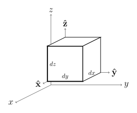
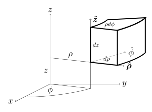
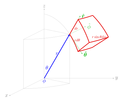
^α θ {\displaystyle \theta } φ {\displaystyle \varphi } θ {\displaystyle \theta } φ {\displaystyle \varphi } mathematical notation . In order to get the mathematics formulae, switch θ {\displaystyle \theta } φ {\displaystyle \varphi } ^β ∂ i A ⊗ e i {\displaystyle \partial _{i}\mathbf {A} \otimes \mathbf {e} _{i}} e i ⊗ ∂ i A {\displaystyle \mathbf {e} _{i}\otimes \partial _{i}\mathbf {A} } ^γ e i ⋅ ∂ i T {\displaystyle \mathbf {e} _{i}\cdot \partial _{i}\mathbf {T} } ∂ i T ⋅ e i {\displaystyle \partial _{i}\mathbf {T} \cdot \mathbf {e} _{i}} Differential elements Operation Cartesian coordinates (x , y , z ) Cylindrical coordinates (ρ , φ , z ) Spherical coordinates α (r , θ , φ ) Differential displacement dℓ [ 1] d x x ^ + d y y ^ + d z z ^ {\displaystyle dx\,{\hat {\mathbf {x} }}+dy\,{\hat {\mathbf {y} }}+dz\,{\hat {\mathbf {z} }}} d ρ ρ ^ + ρ d φ φ ^ + d z z ^ {\displaystyle d\rho \,{\hat {\boldsymbol {\rho }}}+\rho \,d\varphi \,{\hat {\boldsymbol {\varphi }}}+dz\,{\hat {\mathbf {z} }}} d r r ^ + r d θ θ ^ + r sin θ d φ φ ^ {\displaystyle dr\,{\hat {\mathbf {r} }}+r\,d\theta \,{\hat {\boldsymbol {\theta }}}+r\,\sin \theta \,d\varphi \,{\hat {\boldsymbol {\varphi }}}} Differential normal area d S d y d z x ^ + d x d z y ^ + d x d y z ^ {\displaystyle {\begin{aligned}dy\,dz&\,{\hat {\mathbf {x} }}\\{}+dx\,dz&\,{\hat {\mathbf {y} }}\\{}+dx\,dy&\,{\hat {\mathbf {z} }}\end{aligned}}} ρ d φ d z ρ ^ + d ρ d z φ ^ + ρ d ρ d φ z ^ {\displaystyle {\begin{aligned}\rho \,d\varphi \,dz&\,{\hat {\boldsymbol {\rho }}}\\{}+d\rho \,dz&\,{\hat {\boldsymbol {\varphi }}}\\{}+\rho \,d\rho \,d\varphi &\,{\hat {\mathbf {z} }}\end{aligned}}} r 2 sin θ d θ d φ r ^ + r sin θ d r d φ θ ^ + r d r d θ φ ^ {\displaystyle {\begin{aligned}r^{2}\sin \theta \,d\theta \,d\varphi &\,{\hat {\mathbf {r} }}\\{}+r\sin \theta \,dr\,d\varphi &\,{\hat {\boldsymbol {\theta }}}\\{}+r\,dr\,d\theta &\,{\hat {\boldsymbol {\varphi }}}\end{aligned}}} Differential volume dV [ 1] d x d y d z {\displaystyle dx\,dy\,dz} ρ d ρ d φ d z {\displaystyle \rho \,d\rho \,d\varphi \,dz} r 2 sin θ d r d θ d φ {\displaystyle r^{2}\sin \theta \,dr\,d\theta \,d\varphi }
Calculation rules div grad f ≡ ∇ ⋅ ∇ f ≡ ∇ 2 f {\displaystyle \operatorname {div} \,\operatorname {grad} f\equiv \nabla \cdot \nabla f\equiv \nabla ^{2}f} curl grad f ≡ ∇ × ∇ f = 0 {\displaystyle \operatorname {curl} \,\operatorname {grad} f\equiv \nabla \times \nabla f=\mathbf {0} } div curl A ≡ ∇ ⋅ ( ∇ × A ) = 0 {\displaystyle \operatorname {div} \,\operatorname {curl} \mathbf {A} \equiv \nabla \cdot (\nabla \times \mathbf {A} )=0} curl curl A ≡ ∇ × ( ∇ × A ) = ∇ ( ∇ ⋅ A ) − ∇ 2 A {\displaystyle \operatorname {curl} \,\operatorname {curl} \mathbf {A} \equiv \nabla \times (\nabla \times \mathbf {A} )=\nabla (\nabla \cdot \mathbf {A} )-\nabla ^{2}\mathbf {A} } Lagrange's formula for del)∇ 2 ( f g ) = f ∇ 2 g + 2 ∇ f ⋅ ∇ g + g ∇ 2 f {\displaystyle \nabla ^{2}(fg)=f\nabla ^{2}g+2\nabla f\cdot \nabla g+g\nabla ^{2}f} ∇ 2 ( P ⋅ Q ) = Q ⋅ ∇ 2 P − P ⋅ ∇ 2 Q + 2 ∇ ⋅ [ ( P ⋅ ∇ ) Q + P × ∇ × Q ] {\displaystyle \nabla ^{2}\left(\mathbf {P} \cdot \mathbf {Q} \right)=\mathbf {Q} \cdot \nabla ^{2}\mathbf {P} -\mathbf {P} \cdot \nabla ^{2}\mathbf {Q} +2\nabla \cdot \left[\left(\mathbf {P} \cdot \nabla \right)\mathbf {Q} +\mathbf {P} \times \nabla \times \mathbf {Q} \right]\quad } [ 4] )Cartesian derivation
div A = lim V → 0 ∬ ∂ V A ⋅ d S ∭ V d V = [ A x ( x + d x ) − A x ( x ) ] d y d z + [ A y ( y + d y ) − A y ( y ) ] d x d z + [ A z ( z + d z ) − A z ( z ) ] d x d y d x d y d z = ∂ A x ∂ x + ∂ A y ∂ y + ∂ A z ∂ z {\displaystyle {\begin{aligned}\operatorname {div} \mathbf {A} &=\lim _{V\to 0}{\frac {\iint _{\partial V}\mathbf {A} \cdot d\mathbf {S} }{\iiint _{V}dV}}\\[1ex]&={\frac {\left[A_{x}(x{+}dx)-A_{x}(x)\right]dy\,dz+\left[A_{y}(y{+}dy)-A_{y}(y)\right]dx\,dz+\left[A_{z}(z{+}dz)-A_{z}(z)\right]dx\,dy}{dx\,dy\,dz}}\\&={\frac {\partial A_{x}}{\partial x}}+{\frac {\partial A_{y}}{\partial y}}+{\frac {\partial A_{z}}{\partial z}}\end{aligned}}}
( curl A ) x = lim S ⊥ x ^ → 0 ∫ ∂ S A ⋅ d ℓ ∬ S d S = [ A z ( y + d y ) − A z ( y ) ] d z − [ A y ( z + d z ) − A y ( z ) ] d y d y d z = ∂ A z ∂ y − ∂ A y ∂ z {\displaystyle {\begin{aligned}(\operatorname {curl} \mathbf {A} )_{x}&=\lim _{S^{\perp \mathbf {\hat {x}} }\to 0}{\frac {\int _{\partial S}\mathbf {A} \cdot d\mathbf {\ell } }{\iint _{S}dS}}\\[1ex]&={\frac {\left[A_{z}(y{+}dy)-A_{z}(y)\right]dz-\left[A_{y}(z{+}dz)-A_{y}(z)\right]dy}{dy\,dz}}\\&={\frac {\partial A_{z}}{\partial y}}-{\frac {\partial A_{y}}{\partial z}}\end{aligned}}}
The expressions for ( curl A ) y {\displaystyle (\operatorname {curl} \mathbf {A} )_{y}} ( curl A ) z {\displaystyle (\operatorname {curl} \mathbf {A} )_{z}}
Cylindrical derivation
div A = lim V → 0 ∬ ∂ V A ⋅ d S ∭ V d V = [ A ρ ( ρ + d ρ ) ( ρ + d ρ ) − A ρ ( ρ ) ρ ] d ϕ d z + [ A ϕ ( ϕ + d ϕ ) − A ϕ ( ϕ ) ] d ρ d z + [ A z ( z + d z ) − A z ( z ) ] d ρ ( ρ + d ρ / 2 ) d ϕ ρ d ϕ d ρ d z = 1 ρ ∂ ( ρ A ρ ) ∂ ρ + 1 ρ ∂ A ϕ ∂ ϕ + ∂ A z ∂ z {\displaystyle {\begin{aligned}\operatorname {div} \mathbf {A} &=\lim _{V\to 0}{\frac {\iint _{\partial V}\mathbf {A} \cdot d\mathbf {S} }{\iiint _{V}dV}}\\&={\frac {\left[A_{\rho }(\rho {+}d\rho )(\rho {+}d\rho )-A_{\rho }(\rho )\rho \right]d\phi \,dz+\left[A_{\phi }(\phi {+}d\phi )-A_{\phi }(\phi )\right]d\rho \,dz+\left[A_{z}(z{+}dz)-A_{z}(z)\right]d\rho (\rho {+}d\rho /2)\,d\phi }{\rho \,d\phi \,d\rho \,dz}}\\&={\frac {1}{\rho }}{\frac {\partial (\rho A_{\rho })}{\partial \rho }}+{\frac {1}{\rho }}{\frac {\partial A_{\phi }}{\partial \phi }}+{\frac {\partial A_{z}}{\partial z}}\end{aligned}}}
( curl A ) ρ = lim S ⊥ ρ ^ → 0 ∫ ∂ S A ⋅ d ℓ ∬ S d S = A ϕ ( z ) ( ρ + d ρ ) d ϕ − A ϕ ( z + d z ) ( ρ + d ρ ) d ϕ + A z ( ϕ + d ϕ ) d z − A z ( ϕ ) d z ( ρ + d ρ ) d ϕ d z = − ∂ A ϕ ∂ z + 1 ρ ∂ A z ∂ ϕ {\displaystyle {\begin{aligned}(\operatorname {curl} \mathbf {A} )_{\rho }&=\lim _{S^{\perp {\hat {\boldsymbol {\rho }}}}\to 0}{\frac {\int _{\partial S}\mathbf {A} \cdot d{\boldsymbol {\ell }}}{\iint _{S}dS}}\\[1ex]&={\frac {A_{\phi }(z)\left(\rho +d\rho \right)\,d\phi -A_{\phi }(z+dz)\left(\rho +d\rho \right)\,d\phi +A_{z}(\phi +d\phi )\,dz-A_{z}(\phi )\,dz}{\left(\rho +d\rho \right)\,d\phi \,dz}}\\[1ex]&=-{\frac {\partial A_{\phi }}{\partial z}}+{\frac {1}{\rho }}{\frac {\partial A_{z}}{\partial \phi }}\end{aligned}}}
( curl A ) ϕ = lim S ⊥ ϕ ^ → 0 ∫ ∂ S A ⋅ d ℓ ∬ S d S = A z ( ρ ) d z − A z ( ρ + d ρ ) d z + A ρ ( z + d z ) d ρ − A ρ ( z ) d ρ d ρ d z = − ∂ A z ∂ ρ + ∂ A ρ ∂ z {\displaystyle {\begin{aligned}(\operatorname {curl} \mathbf {A} )_{\phi }&=\lim _{S^{\perp {\boldsymbol {\hat {\phi }}}}\to 0}{\frac {\int _{\partial S}\mathbf {A} \cdot d{\boldsymbol {\ell }}}{\iint _{S}dS}}\\&={\frac {A_{z}(\rho )\,dz-A_{z}(\rho +d\rho )\,dz+A_{\rho }(z+dz)\,d\rho -A_{\rho }(z)\,d\rho }{d\rho \,dz}}\\&=-{\frac {\partial A_{z}}{\partial \rho }}+{\frac {\partial A_{\rho }}{\partial z}}\end{aligned}}}
( curl A ) z = lim S ⊥ z ^ → 0 ∫ ∂ S A ⋅ d ℓ ∬ S d S = A ρ ( ϕ ) d ρ − A ρ ( ϕ + d ϕ ) d ρ + A ϕ ( ρ + d ρ ) ( ρ + d ρ ) d ϕ − A ϕ ( ρ ) ρ d ϕ ρ d ρ d ϕ = − 1 ρ ∂ A ρ ∂ ϕ + 1 ρ ∂ ( ρ A ϕ ) ∂ ρ {\displaystyle {\begin{aligned}(\operatorname {curl} \mathbf {A} )_{z}&=\lim _{S^{\perp {\hat {\boldsymbol {z}}}}\to 0}{\frac {\int _{\partial S}\mathbf {A} \cdot d\mathbf {\ell } }{\iint _{S}dS}}\\[1ex]&={\frac {A_{\rho }(\phi )\,d\rho -A_{\rho }(\phi +d\phi )\,d\rho +A_{\phi }(\rho +d\rho )(\rho +d\rho )\,d\phi -A_{\phi }(\rho )\rho \,d\phi }{\rho \,d\rho \,d\phi }}\\[1ex]&=-{\frac {1}{\rho }}{\frac {\partial A_{\rho }}{\partial \phi }}+{\frac {1}{\rho }}{\frac {\partial (\rho A_{\phi })}{\partial \rho }}\end{aligned}}}
curl A = ( curl A ) ρ ρ ^ + ( curl A ) ϕ ϕ ^ + ( curl A ) z z ^ = ( 1 ρ ∂ A z ∂ ϕ − ∂ A ϕ ∂ z ) ρ ^ + ( ∂ A ρ ∂ z − ∂ A z ∂ ρ ) ϕ ^ + 1 ρ ( ∂ ( ρ A ϕ ) ∂ ρ − ∂ A ρ ∂ ϕ ) z ^ {\displaystyle {\begin{aligned}\operatorname {curl} \mathbf {A} &=(\operatorname {curl} \mathbf {A} )_{\rho }{\hat {\boldsymbol {\rho }}}+(\operatorname {curl} \mathbf {A} )_{\phi }{\hat {\boldsymbol {\phi }}}+(\operatorname {curl} \mathbf {A} )_{z}{\hat {\boldsymbol {z}}}\\[1ex]&=\left({\frac {1}{\rho }}{\frac {\partial A_{z}}{\partial \phi }}-{\frac {\partial A_{\phi }}{\partial z}}\right){\hat {\boldsymbol {\rho }}}+\left({\frac {\partial A_{\rho }}{\partial z}}-{\frac {\partial A_{z}}{\partial \rho }}\right){\hat {\boldsymbol {\phi }}}+{\frac {1}{\rho }}\left({\frac {\partial (\rho A_{\phi })}{\partial \rho }}-{\frac {\partial A_{\rho }}{\partial \phi }}\right){\hat {\boldsymbol {z}}}\end{aligned}}}
Spherical derivation div A = lim V → 0 ∬ ∂ V A ⋅ d S ∭ V d V = [ A r ( r + d r ) ( r + d r ) 2 − A r ( r ) r 2 ] sin θ d θ d ϕ + [ A θ ( θ + d θ ) sin ( θ + d θ ) − A θ ( θ ) sin θ ] r d r d ϕ + [ A ϕ ( ϕ + d ϕ ) − A ϕ ( ϕ ) ] r d r d θ d r r d θ r sin θ d ϕ = 1 r 2 ∂ ( r 2 A r ) ∂ r + 1 r sin θ ∂ ( A θ sin θ ) ∂ θ + 1 r sin θ ∂ A ϕ ∂ ϕ {\displaystyle {\begin{aligned}\operatorname {div} \mathbf {A} &=\lim _{V\to 0}{\frac {\iint _{\partial V}\mathbf {A} \cdot d\mathbf {S} }{\iiint _{V}dV}}\\&={\frac {\left[A_{r}(r{+}dr)(r{+}dr)^{2}-A_{r}(r)r^{2}\right]\sin \theta \,d\theta \,d\phi +\left[A_{\theta }(\theta {+}d\theta )\sin(\theta {+}d\theta )-A_{\theta }(\theta )\sin \theta \right]r\,dr\,d\phi +\left[A_{\phi }(\phi {+}d\phi )-A_{\phi }(\phi )\right]r\,dr\,d\theta }{dr\,r\,d\theta \,r\sin \theta \,d\phi }}\\&={\frac {1}{r^{2}}}{\frac {\partial (r^{2}A_{r})}{\partial r}}+{\frac {1}{r\sin \theta }}{\frac {\partial (A_{\theta }\sin \theta )}{\partial \theta }}+{\frac {1}{r\sin \theta }}{\frac {\partial A_{\phi }}{\partial \phi }}\end{aligned}}}
( curl A ) r = lim S ⊥ r ^ → 0 ∫ ∂ S A ⋅ d ℓ ∬ S d S = A θ ( ϕ ) r d θ + A ϕ ( θ + d θ ) r sin ( θ + d θ ) d ϕ − A θ ( ϕ + d ϕ ) r d θ − A ϕ ( θ ) r sin ( θ ) d ϕ r d θ r sin θ d ϕ = 1 r sin θ ∂ ( A ϕ sin θ ) ∂ θ − 1 r sin θ ∂ A θ ∂ ϕ {\displaystyle {\begin{aligned}(\operatorname {curl} \mathbf {A} )_{r}&=\lim _{S^{\perp {\boldsymbol {\hat {r}}}}\to 0}{\frac {\int _{\partial S}\mathbf {A} \cdot d\mathbf {\ell } }{\iint _{S}dS}}\\[1ex]&={\frac {A_{\theta }(\phi )r\,d\theta +A_{\phi }(\theta +d\theta )r\sin(\theta +d\theta )\,d\phi -A_{\theta }(\phi +d\phi )r\,d\theta -A_{\phi }(\theta )r\sin(\theta )\,d\phi }{r\,d\theta \,r\sin \theta \,d\phi }}\\&={\frac {1}{r\sin \theta }}{\frac {\partial (A_{\phi }\sin \theta )}{\partial \theta }}-{\frac {1}{r\sin \theta }}{\frac {\partial A_{\theta }}{\partial \phi }}\end{aligned}}}
( curl A ) θ = lim S ⊥ θ ^ → 0 ∫ ∂ S A ⋅ d ℓ ∬ S d S = A ϕ ( r ) r sin θ d ϕ + A r ( ϕ + d ϕ ) d r − A ϕ ( r + d r ) ( r + d r ) sin θ d ϕ − A r ( ϕ ) d r d r r sin θ d ϕ = 1 r sin θ ∂ A r ∂ ϕ − 1 r ∂ ( r A ϕ ) ∂ r {\displaystyle {\begin{aligned}(\operatorname {curl} \mathbf {A} )_{\theta }&=\lim _{S^{\perp {\boldsymbol {\hat {\theta }}}}\to 0}{\frac {\int _{\partial S}\mathbf {A} \cdot d\mathbf {\ell } }{\iint _{S}dS}}\\[1ex]&={\frac {A_{\phi }(r)r\sin \theta \,d\phi +A_{r}(\phi +d\phi )\,dr-A_{\phi }(r+dr)(r+dr)\sin \theta \,d\phi -A_{r}(\phi )\,dr}{dr\,r\sin \theta \,d\phi }}\\&={\frac {1}{r\sin \theta }}{\frac {\partial A_{r}}{\partial \phi }}-{\frac {1}{r}}{\frac {\partial (rA_{\phi })}{\partial r}}\end{aligned}}}
( curl A ) ϕ = lim S ⊥ ϕ ^ → 0 ∫ ∂ S A ⋅ d ℓ ∬ S d S = A r ( θ ) d r + A θ ( r + d r ) ( r + d r ) d θ − A r ( θ + d θ ) d r − A θ ( r ) r d θ r d r d θ = 1 r ∂ ( r A θ ) ∂ r − 1 r ∂ A r ∂ θ {\displaystyle {\begin{aligned}(\operatorname {curl} \mathbf {A} )_{\phi }&=\lim _{S^{\perp {\boldsymbol {\hat {\phi }}}}\to 0}{\frac {\int _{\partial S}\mathbf {A} \cdot d\mathbf {\ell } }{\iint _{S}dS}}\\[1ex]&={\frac {A_{r}(\theta )\,dr+A_{\theta }(r+dr)(r+dr)\,d\theta -A_{r}(\theta +d\theta )\,dr-A_{\theta }(r)r\,d\theta }{r\,dr\,d\theta }}\\&={\frac {1}{r}}{\frac {\partial (rA_{\theta })}{\partial r}}-{\frac {1}{r}}{\frac {\partial A_{r}}{\partial \theta }}\end{aligned}}}
curl A = ( curl A ) r r ^ + ( curl A ) θ θ ^ + ( curl A ) ϕ ϕ ^ = 1 r sin θ ( ∂ ( A ϕ sin θ ) ∂ θ − ∂ A θ ∂ ϕ ) r ^ + 1 r ( 1 sin θ ∂ A r ∂ ϕ − ∂ ( r A ϕ ) ∂ r ) θ ^ + 1 r ( ∂ ( r A θ ) ∂ r − ∂ A r ∂ θ ) ϕ ^ {\displaystyle {\begin{aligned}\operatorname {curl} \mathbf {A} &=(\operatorname {curl} \mathbf {A} )_{r}\,{\hat {\boldsymbol {r}}}+(\operatorname {curl} \mathbf {A} )_{\theta }\,{\hat {\boldsymbol {\theta }}}+(\operatorname {curl} \mathbf {A} )_{\phi }\,{\hat {\boldsymbol {\phi }}}\\[1ex]&={\frac {1}{r\sin \theta }}\left({\frac {\partial (A_{\phi }\sin \theta )}{\partial \theta }}-{\frac {\partial A_{\theta }}{\partial \phi }}\right){\hat {\boldsymbol {r}}}+{\frac {1}{r}}\left({\frac {1}{\sin \theta }}{\frac {\partial A_{r}}{\partial \phi }}-{\frac {\partial (rA_{\phi })}{\partial r}}\right){\hat {\boldsymbol {\theta }}}+{\frac {1}{r}}\left({\frac {\partial (rA_{\theta })}{\partial r}}-{\frac {\partial A_{r}}{\partial \theta }}\right){\hat {\boldsymbol {\phi }}}\end{aligned}}}
This page is based on this
Wikipedia article Text is available under the
CC BY-SA 4.0 license; additional terms may apply.
Images, videos and audio are available under their respective licenses.