Derivation of the conjugate gradient method

In numerical linear algebra, the conjugate gradient method is an iterative method for numerically solving the linear system

${\displaystyle {\boldsymbol {Ax}}={\boldsymbol {b}}}$

where ${\displaystyle {\boldsymbol {A}}}$ is symmetric positive-definite, without computing ${\displaystyle {\boldsymbol {A}}^{-1}}$ explicitly. The conjugate gradient method can be derived from several different perspectives, including specialization of the conjugate direction method ^[1] for optimization, and variation of the Arnoldi/Lanczos iteration for eigenvalue problems.

The intent of this article is to document the important steps in these derivations.

Conjugate direction

The conjugate gradient method can be seen as a special case of the conjugate direction method applied to minimization of the quadratic function

${\displaystyle f({\boldsymbol {x}})={\boldsymbol {x}}^{\mathrm {T} }{\boldsymbol {A}}{\boldsymbol {x}}-2{\boldsymbol {b}}^{\mathrm {T} }{\boldsymbol {x}}{\text{.}}}$

which allows us to apply geometric intuition.

Line search

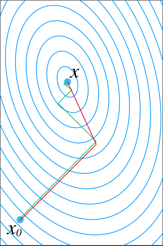
Geometrically, the quadratic function can be equivalently presented by writing down its value at every point in space. The points of equal value make up its contour surfaces, which are concentric ellipsoids with the equation $${\displaystyle {\boldsymbol {x}}^{\mathrm {T} }{\boldsymbol {A}}{\boldsymbol {x}}-2{\boldsymbol {b}}^{\mathrm {T} }{\boldsymbol {x}}=C}$$for varying ${\displaystyle C}$. As ${\displaystyle C}$ decreases, the ellipsoids become smaller and smaller, until at its minimal value, the ellipsoid shrinks to their shared center.

Minimizing the quadratic function is then a problem of moving around the plane, searching for that shared center of all those ellipsoids. The center can be found by computing ${\displaystyle {\boldsymbol {A}}^{-1}}$ explicitly, but this is precisely what we are trying to avoid.

The simplest method is greedy line search, where we start at some point ${\displaystyle {\boldsymbol {x}}_{0}}$, pick a direction ${\displaystyle {\boldsymbol {p}}_{0}}$ somehow, then minimize ${\displaystyle f({\boldsymbol {x}}_{0}+{\boldsymbol {p}}_{0}\alpha _{0})}$. This has a simple closed-form solution that does not involve matrix inversion:$${\displaystyle \alpha _{0}={\frac {{\boldsymbol {p}}_{0}^{\mathrm {T} }({\boldsymbol {b}}-{\boldsymbol {Ax}}_{0})}{{\boldsymbol {p}}_{0}^{\mathrm {T} }{\boldsymbol {A}}{\boldsymbol {p}}_{0}}}}$$Geometrically, we start at some point ${\displaystyle {\boldsymbol {x}}_{0}}$ on some ellipsoid, then choose a direction and travel along that direction, until we hit the point where the ellipsoid is minimized in that direction. This is not necessarily the minimum, but it is progress towards it. Visually, it is moving along a line, and stopping as soon as we reach a point tangent to the contour ellipsoid.

We can now repeat this procedure, starting at our new point ${\displaystyle {\boldsymbol {x}}_{1}={\boldsymbol {x}}_{0}+\alpha _{0}{\boldsymbol {p}}_{0}}$, pick a new direction ${\displaystyle {\boldsymbol {p}}_{1}}$, compute ${\displaystyle \alpha _{1}}$, etc.

We can summarize this as the following algorithm:

Start by picking an initial guess ${\displaystyle {\boldsymbol {x}}_{0}}$, and compute the initial residual ${\displaystyle {\boldsymbol {r}}_{0}={\boldsymbol {b}}-{\boldsymbol {Ax}}_{0}}$, then iterate:

${\displaystyle {\begin{aligned}\alpha _{i}&={\frac {{\boldsymbol {p}}_{i}^{\mathrm {T} }{\boldsymbol {r}}_{i}}{{\boldsymbol {p}}_{i}^{\mathrm {T} }{\boldsymbol {Ap}}_{i}}}{\text{,}}\\{\boldsymbol {x}}_{i+1}&={\boldsymbol {x}}_{i}+\alpha _{i}{\boldsymbol {p}}_{i}{\text{,}}\\{\boldsymbol {r}}_{i+1}&={\boldsymbol {r}}_{i}-\alpha _{i}{\boldsymbol {Ap}}_{i}\end{aligned}}}$

where ${\displaystyle {\boldsymbol {p}}_{0},{\boldsymbol {p}}_{1},{\boldsymbol {p}}_{2},\ldots }$ are to be picked. Notice in particular how the residual is calculated iteratively step-by-step, instead of anew every time:$${\displaystyle {\boldsymbol {r}}_{i+1}={\boldsymbol {b}}-{\boldsymbol {Ax}}_{i+1}={\boldsymbol {b}}-{\boldsymbol {A}}({\boldsymbol {x}}_{i}+\alpha _{i}{\boldsymbol {p}}_{i})={\boldsymbol {r}}_{i}-\alpha _{i}{\boldsymbol {A}}{\boldsymbol {p}}_{i}}$$It is possibly true that ${\displaystyle \alpha _{i}=0}$ prematurely, which would bring numerical problems. However, for particular choices of ${\displaystyle {\boldsymbol {p}}_{0},{\boldsymbol {p}}_{1},{\boldsymbol {p}}_{2},\ldots }$, this will not occur before convergence, as we will prove below.

Conjugate directions

If the directions ${\displaystyle {\boldsymbol {p}}_{0},{\boldsymbol {p}}_{1},{\boldsymbol {p}}_{2},\ldots }$ are not picked well, then progress will be slow. In particular, the gradient descent method would be slow. This can be seen in the diagram, where the green line is the result of always picking the local gradient direction. It zig-zags towards the minimum, but repeatedly overshoots. In contrast, if we pick the directions to be a set of mutually conjugate directions, then there will be no overshoot, and we would obtain the global minimum after ${\displaystyle n}$ steps, where ${\displaystyle n}$ is the number of dimensions.

Two conjugate diameters of an ellipse. Each edge of the bounding parallelogram is parallel to one of the diameters.

The concept of conjugate directions came from classical geometry of ellipse. For an ellipse, two semi-axes center are mutually conjugate with respect to the ellipse iff the lines are parallel to the tangent bounding parallelogram, as pictured. The concept generalizes to n-dimensional ellipsoids, where n semi-axes ${\displaystyle t_{0}{\boldsymbol {p}}_{0},\dots ,t_{n-1}{\boldsymbol {p}}_{n-1}}$ are mutually conjugate with respect to the ellipsoid iff each axis is parallel to the tangent bounding parallelepiped. In other words, for any ${\displaystyle i}$, the tangent plane to the ellipsoid at ${\displaystyle {\boldsymbol {c}}+t_{i}{\boldsymbol {p}}_{i}}$ is a hyperplane spanned by the vectors ${\displaystyle \{{\boldsymbol {p}}_{j}:j\neq i\}}$, where ${\displaystyle {\boldsymbol {c}}}$ is the center of the ellipsoid.

Note that we need to scale each directional vector ${\displaystyle {\boldsymbol {p}}_{i}}$ by a scalar ${\displaystyle t_{i}}$, so that ${\displaystyle {\boldsymbol {c}}+t_{i}{\boldsymbol {p}}_{i}}$ falls exactly on the ellipsoid.

Given an ellipsoid with equation $${\displaystyle {\boldsymbol {x}}^{\mathrm {T} }{\boldsymbol {A}}{\boldsymbol {x}}-2{\boldsymbol {b}}^{\mathrm {T} }{\boldsymbol {x}}=C}$$for some constant ${\displaystyle C}$, we can translate it so that its center is at origin. This changes the equation to $${\displaystyle {\boldsymbol {x}}^{\mathrm {T} }{\boldsymbol {A}}{\boldsymbol {x}}=C'}$$for some other constant ${\displaystyle C'}$. The condition of tangency is then:$${\displaystyle (t_{i}{\boldsymbol {p}}_{i}+{\boldsymbol {p}}_{j}dt_{j})^{\mathrm {T} }{\boldsymbol {A}}(t_{i}{\boldsymbol {p}}_{i}+{\boldsymbol {p}}_{j}dt_{j})=C'+O(dt_{j}^{2}),\quad \forall i\neq j}$$that is, ${\displaystyle {\boldsymbol {p}}_{i}^{\mathrm {T} }{\boldsymbol {Ap}}_{j}=0}$ for any ${\displaystyle i\neq j}$.

The conjugate direction method is imprecise in the sense that no formulae are given for selection of the directions ${\displaystyle {\boldsymbol {p}}_{0},{\boldsymbol {p}}_{1},{\boldsymbol {p}}_{2},\ldots }$. Specific choices lead to various methods including the conjugate gradient method and Gaussian elimination.

Gram–Schmidt process

We can tabulate the equations that we need to set to zero:

	0	1	2	3	${\displaystyle \cdots }$
0		${\displaystyle {\boldsymbol {p}}_{0}^{\mathrm {T} }{\boldsymbol {Ap}}_{1}}$	${\displaystyle {\boldsymbol {p}}_{0}^{\mathrm {T} }{\boldsymbol {Ap}}_{2}}$	${\displaystyle {\boldsymbol {p}}_{0}^{\mathrm {T} }{\boldsymbol {Ap}}_{3}}$	${\displaystyle \cdots }$
1			${\displaystyle {\boldsymbol {p}}_{1}^{\mathrm {T} }{\boldsymbol {Ap}}_{2}}$	${\displaystyle {\boldsymbol {p}}_{1}^{\mathrm {T} }{\boldsymbol {Ap}}_{3}}$	${\displaystyle \cdots }$
2				${\displaystyle {\boldsymbol {p}}_{2}^{\mathrm {T} }{\boldsymbol {Ap}}_{3}}$	${\displaystyle \cdots }$
${\displaystyle \vdots }$					${\displaystyle \ddots }$

This resembles the problem of orthogonalization, which requires ${\displaystyle {\boldsymbol {p}}_{i}^{\mathrm {T} }{\boldsymbol {p}}_{j}=0}$ for any ${\displaystyle i\neq j}$, and ${\displaystyle {\boldsymbol {p}}_{i}^{\mathrm {T} }{\boldsymbol {p}}_{j}=1}$ for any ${\displaystyle i=j}$. Thus the problem of finding conjugate axes is less constrained than the problem of orthogonalization, so the Gram–Schmidt process works, with additional degrees of freedom that we can later use to pick the ones that would simplify the computation:

• Arbitrarily set ${\displaystyle {\boldsymbol {p}}_{0}}$.
• Arbitrarily set ${\displaystyle {\boldsymbol {p}}_{10}}$, then modify it to ${\displaystyle {\boldsymbol {p}}_{1}={\boldsymbol {p}}_{10}-{\frac {{\boldsymbol {p}}_{0}^{\mathrm {T} }{\boldsymbol {Ap}}_{10}}{{\boldsymbol {p}}_{0}^{\mathrm {T} }{\boldsymbol {Ap}}_{0}}}{\boldsymbol {p}}_{0}}$.
• Arbitrarily set ${\displaystyle {\boldsymbol {p}}_{20}}$, then modify it to ${\displaystyle {\boldsymbol {p}}_{2}={\boldsymbol {p}}_{20}-\sum _{i=0}^{1}{\frac {{\boldsymbol {p}}_{i}^{\mathrm {T} }{\boldsymbol {Ap}}_{20}}{{\boldsymbol {p}}_{i}^{\mathrm {T} }{\boldsymbol {Ap}}_{i}}}{\boldsymbol {p}}_{i}}$.
• ...
• Arbitrarily set ${\displaystyle {\boldsymbol {p}}_{n-1,0}}$, then modify it to ${\displaystyle {\boldsymbol {p}}_{n-1}={\boldsymbol {p}}_{n-1,0}-\sum _{i=0}^{n-2}{\frac {{\boldsymbol {p}}_{i}^{\mathrm {T} }{\boldsymbol {Ap}}_{n-1,0}}{{\boldsymbol {p}}_{i}^{\mathrm {T} }{\boldsymbol {Ap}}_{i}}}{\boldsymbol {p}}_{i}}$.

The most natural choice of ${\displaystyle {\boldsymbol {p}}_{k,0}}$ is the gradient. That is, ${\displaystyle {\boldsymbol {p}}_{k,0}=\nabla f({\boldsymbol {x}}_{k})}$. Since conjugate directions can be scaled by a nonzero value, we scale it by ${\displaystyle -1/2}$ for notational cleanness, obtaining $${\displaystyle {\boldsymbol {p}}_{k,0}=\mathbf {r} _{k}=\mathbf {b} -\mathbf {Ax} _{k}}$$Thus, we have ${\displaystyle {\boldsymbol {p}}_{k}={\boldsymbol {r}}_{k}-\sum _{i=0}^{k-1}{\frac {{\boldsymbol {p}}_{i}^{\mathrm {T} }{\boldsymbol {Ar}}_{k}}{{\boldsymbol {p}}_{i}^{\mathrm {T} }{\boldsymbol {Ap}}_{i}}}{\boldsymbol {p}}_{i}}$. Plugging it in, we have the conjugate gradient algorithm:$${\displaystyle {\begin{aligned}&\mathbf {r} _{0}:=\mathbf {b} -\mathbf {Ax} _{0}\\&\mathbf {p} _{0}:=\mathbf {r} _{0}\\&k:=0\\&{\text{do while }}k<n\\&\qquad \alpha _{k}:={\frac {\mathbf {p} _{k}^{\mathsf {T}}\mathbf {r} _{k}}{\mathbf {p} _{k}^{\mathsf {T}}\mathbf {Ap} _{k}}}\\&\qquad \mathbf {x} _{k+1}:=\mathbf {x} _{k}+\alpha _{k}\mathbf {p} _{k}\\&\qquad {\text{if }}|\alpha _{k}|{\text{ is sufficiently small, then exit loop}}\\&\qquad \mathbf {r} _{k+1}:=\mathbf {r} _{k}-\alpha _{k}\mathbf {Ap} _{k}\\&\qquad \mathbf {p} _{k+1}:={\boldsymbol {r}}_{k+1}-\sum _{i=0}^{k}{\frac {{\boldsymbol {p}}_{i}^{\mathrm {T} }{\boldsymbol {Ar}}_{k+1}}{{\boldsymbol {p}}_{i}^{\mathrm {T} }{\boldsymbol {Ap}}_{i}}}{\boldsymbol {p}}_{i}\\&\qquad k:=k+1\\&{\text{return }}\mathbf {x} _{k+1}{\text{ as the result}}\end{aligned}}}$$Proposition. If at some point, ${\displaystyle \alpha _{k}=0}$, then the algorithm has converged, that is, ${\displaystyle \nabla f(\mathrm {x} _{k+1})=0}$.

Proof. By construction, it would mean that ${\displaystyle \mathbf {x} _{k+1}=\mathbf {x} _{k}}$, that is, taking a conjugate gradient step gets us exactly back to where we were. This is only possible if the local gradient is already zero.

Simplification

This algorithm can be significantly simplified by some lemmas, resulting in the conjugate gradient algorithm.

Lemma 1.${\displaystyle \mathbf {p} _{i}^{T}\mathbf {r} _{j}=0,\;\forall i<j}$ and ${\displaystyle \mathbf {r} _{i}^{T}\mathbf {r} _{j}=0,\;\forall i<j}$.

Proof. By the geometric construction, the tangent plane to the ellipsoid at ${\displaystyle \mathbf {x} _{j}}$ contains each of the previous conjugate direction vectors ${\displaystyle \mathbf {p} _{0},\mathbf {p} _{1},\dots ,\mathbf {p} _{j-1}}$. Further, ${\displaystyle \mathbf {r} _{j}}$ is perpendicular to the tangent, thus ${\displaystyle \mathbf {p} _{i}^{T}\mathbf {r} _{j}=0,\;\forall i<j}$. The second equation is true since by construction, ${\displaystyle \mathbf {r} _{0},\mathbf {r} _{1},\dots ,\mathbf {r} _{j-1}}$ is a linear transform of ${\displaystyle \mathbf {p} _{0},\mathbf {p} _{1},\dots ,\mathbf {p} _{j-1}}$.

Lemma 2.${\displaystyle \mathbf {p} _{k}^{T}\mathbf {r} _{k}=\mathbf {r} _{k}^{T}\mathbf {r} _{k}}$.

Proof. By construction, ${\displaystyle \mathbf {p} _{k}:={\boldsymbol {r}}_{k}-\sum _{i=0}^{k-1}{\frac {{\boldsymbol {p}}_{i}^{\mathrm {T} }{\boldsymbol {Ar}}_{k-1}}{{\boldsymbol {p}}_{i}^{\mathrm {T} }{\boldsymbol {Ap}}_{i}}}{\boldsymbol {p}}_{i}}$, now apply lemma 1.

Lemma 3.${\displaystyle {\boldsymbol {p}}_{i}^{\mathrm {T} }{\boldsymbol {Ar}}_{k+1}={\begin{cases}0,\;i<k\\-{\boldsymbol {r}}_{k+1}^{T}{\boldsymbol {r}}_{k+1}/\alpha _{k},\;i=k\end{cases}}}$.

Proof. By construction, we have ${\displaystyle \mathbf {r} _{i+1}=\mathbf {r} _{i}-\alpha _{k}\mathbf {Ap} _{i}}$, thus$${\displaystyle {\boldsymbol {r}}_{k+1}^{T}{\boldsymbol {A}}{\boldsymbol {p}}_{i}={\boldsymbol {r}}_{k+1}^{T}{\frac {{\boldsymbol {r}}_{i}-{\boldsymbol {r}}_{i+1}}{\alpha _{i}}}}$$Now apply lemma 1.

Plugging lemmas 1-3 in, we have ${\displaystyle \alpha _{k}={\frac {\mathbf {r} _{k}^{\top }\mathbf {r} _{k}}{\mathbf {p} _{k}^{\top }\mathbf {A} \mathbf {p} _{k}}}}$ and ${\displaystyle \mathbf {p} _{k+1}:={\boldsymbol {r}}_{k+1}+{\frac {\mathbf {r} _{k+1}^{\top }\mathbf {r} _{k+1}}{\mathbf {r} _{k}^{\top }\mathbf {r} _{k}}}\mathbf {p} _{k}}$, which is the proper conjugate gradient algorithm.

Arnoldi/Lanczos iteration

Further information: Arnoldi iteration and Lanczos iteration

The conjugate gradient method can also be seen as a variant of the Arnoldi/Lanczos iteration applied to solving linear systems.

The general Arnoldi method

In the Arnoldi iteration, one starts with a vector ${\displaystyle {\boldsymbol {r}}_{0}}$ and gradually builds an orthonormal basis ${\displaystyle \{{\boldsymbol {v}}_{1},{\boldsymbol {v}}_{2},{\boldsymbol {v}}_{3},\ldots \}}$ of the Krylov subspace

${\displaystyle {\mathcal {K}}({\boldsymbol {A}},{\boldsymbol {r}}_{0})=\mathrm {span} \{{\boldsymbol {r}}_{0},{\boldsymbol {Ar}}_{0},{\boldsymbol {A}}^{2}{\boldsymbol {r}}_{0},\ldots \}}$

by defining ${\displaystyle {\boldsymbol {v}}_{i}={\boldsymbol {w}}_{i}/\lVert {\boldsymbol {w}}_{i}\rVert _{2}}$ where

${\displaystyle {\boldsymbol {v}}_{i}={\begin{cases}{\boldsymbol {r}}_{0}&{\text{if }}i=1{\text{,}}\\{\boldsymbol {Av}}_{i-1}-\sum _{j=1}^{i-1}({\boldsymbol {v}}_{j}^{\mathrm {T} }{\boldsymbol {Av}}_{i-1}){\boldsymbol {v}}_{j}&{\text{if }}i>1{\text{.}}\end{cases}}}$

In other words, for ${\displaystyle i>1}$, ${\displaystyle {\boldsymbol {v}}_{i}}$ is found by Gram-Schmidt orthogonalizing ${\displaystyle {\boldsymbol {Av}}_{i-1}}$ against ${\displaystyle \{{\boldsymbol {v}}_{1},{\boldsymbol {v}}_{2},\ldots ,{\boldsymbol {v}}_{i-1}\}}$ followed by normalization.

Put in matrix form, the iteration is captured by the equation

${\displaystyle {\boldsymbol {AV}}_{i}={\boldsymbol {V}}_{i+1}{\boldsymbol {\tilde {H}}}_{i}}$

where

${\displaystyle {\begin{aligned}{\boldsymbol {V}}_{i}&={\begin{bmatrix}{\boldsymbol {v}}_{1}&{\boldsymbol {v}}_{2}&\cdots &{\boldsymbol {v}}_{i}\end{bmatrix}}{\text{,}}\\{\boldsymbol {\tilde {H}}}_{i}&={\begin{bmatrix}h_{11}&h_{12}&h_{13}&\cdots &h_{1,i}\\h_{21}&h_{22}&h_{23}&\cdots &h_{2,i}\\&h_{32}&h_{33}&\cdots &h_{3,i}\\&&\ddots &\ddots &\vdots \\&&&h_{i,i-1}&h_{i,i}\\&&&&h_{i+1,i}\end{bmatrix}}={\begin{bmatrix}{\boldsymbol {H}}_{i}\\h_{i+1,i}{\boldsymbol {e}}_{i}^{\mathrm {T} }\end{bmatrix}}\end{aligned}}}$

with

${\displaystyle h_{ji}={\begin{cases}{\boldsymbol {v}}_{j}^{\mathrm {T} }{\boldsymbol {Av}}_{i}&{\text{if }}j\leq i{\text{,}}\\\lVert {\boldsymbol {w}}_{i+1}\rVert _{2}&{\text{if }}j=i+1{\text{,}}\\0&{\text{if }}j>i+1{\text{.}}\end{cases}}}$

When applying the Arnoldi iteration to solving linear systems, one starts with ${\displaystyle {\boldsymbol {r}}_{0}={\boldsymbol {b}}-{\boldsymbol {Ax}}_{0}}$, the residual corresponding to an initial guess ${\displaystyle {\boldsymbol {x}}_{0}}$. After each step of iteration, one computes ${\displaystyle {\boldsymbol {y}}_{i}={\boldsymbol {H}}_{i}^{-1}(\lVert {\boldsymbol {r}}_{0}\rVert _{2}{\boldsymbol {e}}_{1})}$ and the new iterate ${\displaystyle {\boldsymbol {x}}_{i}={\boldsymbol {x}}_{0}+{\boldsymbol {V}}_{i}{\boldsymbol {y}}_{i}}$.

The direct Lanczos method

For the rest of discussion, we assume that ${\displaystyle {\boldsymbol {A}}}$ is symmetric positive-definite. With symmetry of ${\displaystyle {\boldsymbol {A}}}$, the upper Hessenberg matrix ${\displaystyle {\boldsymbol {H}}_{i}={\boldsymbol {V}}_{i}^{\mathrm {T} }{\boldsymbol {AV}}_{i}}$ becomes symmetric and thus tridiagonal. It then can be more clearly denoted by

${\displaystyle {\boldsymbol {H}}_{i}={\begin{bmatrix}a_{1}&b_{2}\\b_{2}&a_{2}&b_{3}\\&\ddots &\ddots &\ddots \\&&b_{i-1}&a_{i-1}&b_{i}\\&&&b_{i}&a_{i}\end{bmatrix}}{\text{.}}}$

This enables a short three-term recurrence for ${\displaystyle {\boldsymbol {v}}_{i}}$ in the iteration, and the Arnoldi iteration is reduced to the Lanczos iteration.

Since ${\displaystyle {\boldsymbol {A}}}$ is symmetric positive-definite, so is ${\displaystyle {\boldsymbol {H}}_{i}}$. Hence, ${\displaystyle {\boldsymbol {H}}_{i}}$ can be LU factorized without partial pivoting into

${\displaystyle {\boldsymbol {H}}_{i}={\boldsymbol {L}}_{i}{\boldsymbol {U}}_{i}={\begin{bmatrix}1\\c_{2}&1\\&\ddots &\ddots \\&&c_{i-1}&1\\&&&c_{i}&1\end{bmatrix}}{\begin{bmatrix}d_{1}&b_{2}\\&d_{2}&b_{3}\\&&\ddots &\ddots \\&&&d_{i-1}&b_{i}\\&&&&d_{i}\end{bmatrix}}}$

with convenient recurrences for ${\displaystyle c_{i}}$ and ${\displaystyle d_{i}}$:

${\displaystyle {\begin{aligned}c_{i}&=b_{i}/d_{i-1}{\text{,}}\\d_{i}&={\begin{cases}a_{1}&{\text{if }}i=1{\text{,}}\\a_{i}-c_{i}b_{i}&{\text{if }}i>1{\text{.}}\end{cases}}\end{aligned}}}$

Rewrite ${\displaystyle {\boldsymbol {x}}_{i}={\boldsymbol {x}}_{0}+{\boldsymbol {V}}_{i}{\boldsymbol {y}}_{i}}$ as

${\displaystyle {\begin{aligned}{\boldsymbol {x}}_{i}&={\boldsymbol {x}}_{0}+{\boldsymbol {V}}_{i}{\boldsymbol {H}}_{i}^{-1}(\lVert {\boldsymbol {r}}_{0}\rVert _{2}{\boldsymbol {e}}_{1})\\&={\boldsymbol {x}}_{0}+{\boldsymbol {V}}_{i}{\boldsymbol {U}}_{i}^{-1}{\boldsymbol {L}}_{i}^{-1}(\lVert {\boldsymbol {r}}_{0}\rVert _{2}{\boldsymbol {e}}_{1})\\&={\boldsymbol {x}}_{0}+{\boldsymbol {P}}_{i}{\boldsymbol {z}}_{i}\end{aligned}}}$

with

${\displaystyle {\begin{aligned}{\boldsymbol {P}}_{i}&={\boldsymbol {V}}_{i}{\boldsymbol {U}}_{i}^{-1}{\text{,}}\\{\boldsymbol {z}}_{i}&={\boldsymbol {L}}_{i}^{-1}(\lVert {\boldsymbol {r}}_{0}\rVert _{2}{\boldsymbol {e}}_{1}){\text{.}}\end{aligned}}}$

It is now important to observe that

${\displaystyle {\begin{aligned}{\boldsymbol {P}}_{i}&={\begin{bmatrix}{\boldsymbol {P}}_{i-1}&{\boldsymbol {p}}_{i}\end{bmatrix}}{\text{,}}\\{\boldsymbol {z}}_{i}&={\begin{bmatrix}{\boldsymbol {z}}_{i-1}\\\zeta _{i}\end{bmatrix}}{\text{.}}\end{aligned}}}$

In fact, there are short recurrences for ${\displaystyle {\boldsymbol {p}}_{i}}$ and ${\displaystyle \zeta _{i}}$ as well:

${\displaystyle {\begin{aligned}{\boldsymbol {p}}_{i}&={\frac {1}{d_{i}}}({\boldsymbol {v}}_{i}-b_{i}{\boldsymbol {p}}_{i-1}){\text{,}}\\\zeta _{i}&=-c_{i}\zeta _{i-1}{\text{.}}\end{aligned}}}$

With this formulation, we arrive at a simple recurrence for ${\displaystyle {\boldsymbol {x}}_{i}}$:

${\displaystyle {\begin{aligned}{\boldsymbol {x}}_{i}&={\boldsymbol {x}}_{0}+{\boldsymbol {P}}_{i}{\boldsymbol {z}}_{i}\\&={\boldsymbol {x}}_{0}+{\boldsymbol {P}}_{i-1}{\boldsymbol {z}}_{i-1}+\zeta _{i}{\boldsymbol {p}}_{i}\\&={\boldsymbol {x}}_{i-1}+\zeta _{i}{\boldsymbol {p}}_{i}{\text{.}}\end{aligned}}}$

The relations above straightforwardly lead to the direct Lanczos method, which turns out to be slightly more complex.

The conjugate gradient method from imposing orthogonality and conjugacy

If we allow ${\displaystyle {\boldsymbol {p}}_{i}}$ to scale and compensate for the scaling in the constant factor, we potentially can have simpler recurrences of the form:

${\displaystyle {\begin{aligned}{\boldsymbol {x}}_{i}&={\boldsymbol {x}}_{i-1}+\alpha _{i-1}{\boldsymbol {p}}_{i-1}{\text{,}}\\{\boldsymbol {r}}_{i}&={\boldsymbol {r}}_{i-1}-\alpha _{i-1}{\boldsymbol {Ap}}_{i-1}{\text{,}}\\{\boldsymbol {p}}_{i}&={\boldsymbol {r}}_{i}+\beta _{i-1}{\boldsymbol {p}}_{i-1}{\text{.}}\end{aligned}}}$

As premises for the simplification, we now derive the orthogonality of ${\displaystyle {\boldsymbol {r}}_{i}}$ and conjugacy of ${\displaystyle {\boldsymbol {p}}_{i}}$, i.e., for ${\displaystyle i\neq j}$,

${\displaystyle {\begin{aligned}{\boldsymbol {r}}_{i}^{\mathrm {T} }{\boldsymbol {r}}_{j}&=0{\text{,}}\\{\boldsymbol {p}}_{i}^{\mathrm {T} }{\boldsymbol {Ap}}_{j}&=0{\text{.}}\end{aligned}}}$

The residuals are mutually orthogonal because ${\displaystyle {\boldsymbol {r}}_{i}}$ is essentially a multiple of ${\displaystyle {\boldsymbol {v}}_{i+1}}$ since for ${\displaystyle i=0}$, ${\displaystyle {\boldsymbol {r}}_{0}=\lVert {\boldsymbol {r}}_{0}\rVert _{2}{\boldsymbol {v}}_{1}}$, for ${\displaystyle i>0}$,

${\displaystyle {\begin{aligned}{\boldsymbol {r}}_{i}&={\boldsymbol {b}}-{\boldsymbol {Ax}}_{i}\\&={\boldsymbol {b}}-{\boldsymbol {A}}({\boldsymbol {x}}_{0}+{\boldsymbol {V}}_{i}{\boldsymbol {y}}_{i})\\&={\boldsymbol {r}}_{0}-{\boldsymbol {AV}}_{i}{\boldsymbol {y}}_{i}\\&={\boldsymbol {r}}_{0}-{\boldsymbol {V}}_{i+1}{\boldsymbol {\tilde {H}}}_{i}{\boldsymbol {y}}_{i}\\&={\boldsymbol {r}}_{0}-{\boldsymbol {V}}_{i}{\boldsymbol {H}}_{i}{\boldsymbol {y}}_{i}-h_{i+1,i}({\boldsymbol {e}}_{i}^{\mathrm {T} }{\boldsymbol {y}}_{i}){\boldsymbol {v}}_{i+1}\\&=\lVert {\boldsymbol {r}}_{0}\rVert _{2}{\boldsymbol {v}}_{1}-{\boldsymbol {V}}_{i}(\lVert {\boldsymbol {r}}_{0}\rVert _{2}{\boldsymbol {e}}_{1})-h_{i+1,i}({\boldsymbol {e}}_{i}^{\mathrm {T} }{\boldsymbol {y}}_{i}){\boldsymbol {v}}_{i+1}\\&=-h_{i+1,i}({\boldsymbol {e}}_{i}^{\mathrm {T} }{\boldsymbol {y}}_{i}){\boldsymbol {v}}_{i+1}{\text{.}}\end{aligned}}}$

To see the conjugacy of ${\displaystyle {\boldsymbol {p}}_{i}}$, it suffices to show that ${\displaystyle {\boldsymbol {P}}_{i}^{\mathrm {T} }{\boldsymbol {AP}}_{i}}$ is diagonal:

${\displaystyle {\begin{aligned}{\boldsymbol {P}}_{i}^{\mathrm {T} }{\boldsymbol {AP}}_{i}&={\boldsymbol {U}}_{i}^{-\mathrm {T} }{\boldsymbol {V}}_{i}^{\mathrm {T} }{\boldsymbol {AV}}_{i}{\boldsymbol {U}}_{i}^{-1}\\&={\boldsymbol {U}}_{i}^{-\mathrm {T} }{\boldsymbol {H}}_{i}{\boldsymbol {U}}_{i}^{-1}\\&={\boldsymbol {U}}_{i}^{-\mathrm {T} }{\boldsymbol {L}}_{i}{\boldsymbol {U}}_{i}{\boldsymbol {U}}_{i}^{-1}\\&={\boldsymbol {U}}_{i}^{-\mathrm {T} }{\boldsymbol {L}}_{i}\end{aligned}}}$

is symmetric and lower triangular simultaneously and thus must be diagonal.

Now we can derive the constant factors ${\displaystyle \alpha _{i}}$ and ${\displaystyle \beta _{i}}$ with respect to the scaled ${\displaystyle {\boldsymbol {p}}_{i}}$ by solely imposing the orthogonality of ${\displaystyle {\boldsymbol {r}}_{i}}$ and conjugacy of ${\displaystyle {\boldsymbol {p}}_{i}}$.

Due to the orthogonality of ${\displaystyle {\boldsymbol {r}}_{i}}$, it is necessary that ${\displaystyle {\boldsymbol {r}}_{i+1}^{\mathrm {T} }{\boldsymbol {r}}_{i}=({\boldsymbol {r}}_{i}-\alpha _{i}{\boldsymbol {Ap}}_{i})^{\mathrm {T} }{\boldsymbol {r}}_{i}=0}$. As a result,

${\displaystyle {\begin{aligned}\alpha _{i}&={\frac {{\boldsymbol {r}}_{i}^{\mathrm {T} }{\boldsymbol {r}}_{i}}{{\boldsymbol {r}}_{i}^{\mathrm {T} }{\boldsymbol {Ap}}_{i}}}\\&={\frac {{\boldsymbol {r}}_{i}^{\mathrm {T} }{\boldsymbol {r}}_{i}}{({\boldsymbol {p}}_{i}-\beta _{i-1}{\boldsymbol {p}}_{i-1})^{\mathrm {T} }{\boldsymbol {Ap}}_{i}}}\\&={\frac {{\boldsymbol {r}}_{i}^{\mathrm {T} }{\boldsymbol {r}}_{i}}{{\boldsymbol {p}}_{i}^{\mathrm {T} }{\boldsymbol {Ap}}_{i}}}{\text{.}}\end{aligned}}}$

Similarly, due to the conjugacy of ${\displaystyle {\boldsymbol {p}}_{i}}$, it is necessary that ${\displaystyle {\boldsymbol {p}}_{i+1}^{\mathrm {T} }{\boldsymbol {Ap}}_{i}=({\boldsymbol {r}}_{i+1}+\beta _{i}{\boldsymbol {p}}_{i})^{\mathrm {T} }{\boldsymbol {Ap}}_{i}=0}$. As a result,

${\displaystyle {\begin{aligned}\beta _{i}&=-{\frac {{\boldsymbol {r}}_{i+1}^{\mathrm {T} }{\boldsymbol {Ap}}_{i}}{{\boldsymbol {p}}_{i}^{\mathrm {T} }{\boldsymbol {Ap}}_{i}}}\\&=-{\frac {{\boldsymbol {r}}_{i+1}^{\mathrm {T} }({\boldsymbol {r}}_{i}-{\boldsymbol {r}}_{i+1})}{\alpha _{i}{\boldsymbol {p}}_{i}^{\mathrm {T} }{\boldsymbol {Ap}}_{i}}}\\&={\frac {{\boldsymbol {r}}_{i+1}^{\mathrm {T} }{\boldsymbol {r}}_{i+1}}{{\boldsymbol {r}}_{i}^{\mathrm {T} }{\boldsymbol {r}}_{i}}}{\text{.}}\end{aligned}}}$

This completes the derivation.

References

1. Conjugate Direction Methods http://user.it.uu.se/~matsh/opt/f8/node5.html

1. Hestenes, M. R.; Stiefel, E. (December 1952). "Methods of conjugate gradients for solving linear systems" (PDF). Journal of Research of the National Bureau of Standards. 49 (6): 409. doi:10.6028/jres.049.044.
2. Shewchuk, Jonathan Richard. " An introduction to the conjugate gradient method without the agonizing pain ." (1994)
3. Saad, Y. (2003). "Chapter 6: Krylov Subspace Methods, Part I". Iterative methods for sparse linear systems (2nd ed.). SIAM. ISBN   978-0-89871-534-7.