Feature hashing

Last updated

In machine learning, feature hashing, also known as the hashing trick (by analogy to the kernel trick), is a fast and space-efficient way of vectorizing features, i.e. turning arbitrary features into indices in a vector or matrix. [1] [2] It works by applying a hash function to the features and using their hash values as indices directly (after a modulo operation), rather than looking the indices up in an associative array. In addition to its use for encoding non-numeric values, feature hashing can also be used for dimensionality reduction. [2]

Contents

This trick is often attributed to Weinberger et al. (2009), [2] but there exists a much earlier description of this method published by John Moody in 1989. [1]

Motivation

Motivating example

In a typical document classification task, the input to the machine learning algorithm (both during learning and classification) is free text. From this, a bag of words (BOW) representation is constructed: the individual tokens are extracted and counted, and each distinct token in the training set defines a feature (independent variable) of each of the documents in both the training and test sets.

Machine learning algorithms, however, are typically defined in terms of numerical vectors. Therefore, the bags of words for a set of documents is regarded as a term-document matrix where each row is a single document, and each column is a single feature/word; the entry i, j in such a matrix captures the frequency (or weight) of the j'th term of the vocabulary in document i. (An alternative convention swaps the rows and columns of the matrix, but this difference is immaterial.) Typically, these vectors are extremely sparse—according to Zipf's law.

The common approach is to construct, at learning time or prior to that, a dictionary representation of the vocabulary of the training set, and use that to map words to indices. Hash tables and tries are common candidates for dictionary implementation. E.g., the three documents

can be converted, using the dictionary

TermIndex
John1
likes2
to3
watch4
movies5
Mary6
too7
also8
football9

to the term-document matrix

(Punctuation was removed, as is usual in document classification and clustering.)

The problem with this process is that such dictionaries take up a large amount of storage space and grow in size as the training set grows. [3] On the contrary, if the vocabulary is kept fixed and not increased with a growing training set, an adversary may try to invent new words or misspellings that are not in the stored vocabulary so as to circumvent a machine learned filter. To address this challenge, Yahoo! Research attempted to use feature hashing for their spam filters. [4]

Note that the hashing trick isn't limited to text classification and similar tasks at the document level, but can be applied to any problem that involves large (perhaps unbounded) numbers of features.

Mathematical motivation

Mathematically, a token is an element in a finite (or countably infinite) set . Suppose we only need to process a finite corpus, then we can put all tokens appearing in the corpus into , meaning that is finite. However, suppose we want to process all possible words made of the English letters, then is countably infinite.

Most neural networks can only operate on real vector inputs, so we must construct a "dictionary" function .

When is finite, of size , then we can use one-hot encoding to map it into . First, arbitrarily enumerate , then define . In other words, we assign a unique index to each token, then map the token with index to the unit basis vector .

One-hot encoding is easy to interpret, but it requires one to maintain the arbitrary enumeration of . Given a token , to compute , we must find out the index of the token . Thus, to implement efficiently, we need a fast-to-compute bijection , then we have .

In fact, we can relax the requirement slightly: It suffices to have a fast-to-compute injection, then use .

In practice, there is no simple way to construct an efficient injection . However, we do not need a strict injection, but only an approximate injection. That is, when , we should probably have , so that probably.

At this point, we have just specified that should be a hashing function. Thus we reach the idea of feature hashing.

Algorithms

Feature hashing (Weinberger et al. 2009)

The basic feature hashing algorithm presented in (Weinberger et al. 2009) [2] is defined as follows.

First, one specifies two hash functions: the kernel hash, and the sign hash. Next, one defines the feature hashing function:

Finally, extend this feature hashing function to strings of tokens by

where is the set of all finite strings consisting of tokens in . Equivalently,

Geometric properties

We want to say something about the geometric property of , but , by itself, is just a set of tokens, we cannot impose a geometric structure on it except the discrete topology, which is generated by the discrete metric. To make it nicer, we lift it to , and lift from to by linear extension:

There is an infinite sum there, which must be handled at once. There are essentially only two ways to handle infinities. One may impose a metric, then take its completion, to allow well-behaved infinite sums, or one may demand that nothing is actually infinite, only potentially so. Here, we go for the potential-infinity way, by restricting to contain only vectors with finite support: , only finitely many entries of are nonzero. Define an inner product on in the obvious way:

As a side note, if is infinite, then the inner product space is not complete. Taking its completion would get us to a Hilbert space, which allows well-behaved infinite sums.


Now we have an inner product space, with enough structure to describe the geometry of the feature hashing function .

First, we can see why is called a "kernel hash": it allows us to define a kernel by

In the language of the "kernel trick", is the kernel generated by the "feature map"

Note that this is not the feature map we were using, which is . In fact, we have been using another kernel, defined by

The benefit of augmenting the kernel hash with the binary hash is the following theorem, which states that is an isometry "on average".

Theorem (intuitively stated)  If the binary hash is unbiased (meaning that it takes value with equal probability), then is an isometry in expectation:
Proof By linearity of expectation,
Now, , since we assumed is unbiased. So we continue


The above statement and proof interprets the binary hash function not as a deterministic function of type , but as a random binary vector with unbiased entries, meaning that for any .

This is a good intuitive picture, though not rigorous. For a rigorous statement and proof, see [2]

Pseudocode implementation

Instead of maintaining a dictionary, a feature vectorizer that uses the hashing trick can build a vector of a pre-defined length by applying a hash function h to the features (e.g., words), then using the hash values directly as feature indices and updating the resulting vector at those indices. Here, we assume that feature actually means feature vector.

functionhashing_vectorizer(features:arrayofstring,N:integer):x:=newvector[N]forfinfeatures:h:=hash(f)x[hmodN]+=1returnx

Thus, if our feature vector is ["cat","dog","cat"] and hash function is if is "cat" and if is "dog". Let us take the output feature vector dimension (N) to be 4. Then output x will be [0,2,1,0]. It has been suggested that a second, single-bit output hash function ξ be used to determine the sign of the update value, to counter the effect of hash collisions. [2] If such a hash function is used, the algorithm becomes

functionhashing_vectorizer(features:arrayofstring,N:integer):x:=newvector[N]forfinfeatures:h:=hash(f)idx:=hmodNifξ(f)==1:x[idx]+=1else:x[idx]-=1returnx

The above pseudocode actually converts each sample into a vector. An optimized version would instead only generate a stream of pairs and let the learning and prediction algorithms consume such streams; a linear model can then be implemented as a single hash table representing the coefficient vector.

Extensions and variations

Learned feature hashing

Feature hashing generally suffers from hash collision, which means that there exist pairs of different tokens with the same hash: . A machine learning model trained on feature-hashed words would then have difficulty distinguishing and , essentially because is polysemic.

If is rare, then performance degradation is small, as the model could always just ignore the rare case, and pretend all means . However, if both are common, then the degradation can be serious.

To handle this, one can train supervised hashing functions that avoids mapping common tokens to the same feature vectors. [5]

Applications and practical performance

Ganchev and Dredze showed that in text classification applications with random hash functions and several tens of thousands of columns in the output vectors, feature hashing need not have an adverse effect on classification performance, even without the signed hash function. [3]

Weinberger et al. (2009) applied their version of feature hashing to multi-task learning, and in particular, spam filtering, where the input features are pairs (user, feature) so that a single parameter vector captured per-user spam filters as well as a global filter for several hundred thousand users, and found that the accuracy of the filter went up. [2]

Chen et al. (2015) combined the idea of feature hashing and sparse matrix to construct "virtual matrices": large matrices with small storage requirements. The idea is to treat a matrix as a dictionary, with keys in , and values in . Then, as usual in hashed dictionaries, one can use a hash function , and thus represent a matrix as a vector in , no matter how big is. With virtual matrices, they constructed HashedNets, which are large neural networks taking only small amounts of storage. [6]

Implementations

Implementations of the hashing trick are present in:

See also

Related Research Articles

Bra–ket notation, also called Dirac notation, is a notation for linear algebra and linear operators on complex vector spaces together with their dual space both in the finite-dimensional and infinite-dimensional case. It is specifically designed to ease the types of calculations that frequently come up in quantum mechanics. Its use in quantum mechanics is quite widespread.

The Riesz representation theorem, sometimes called the Riesz–Fréchet representation theorem after Frigyes Riesz and Maurice René Fréchet, establishes an important connection between a Hilbert space and its continuous dual space. If the underlying field is the real numbers, the two are isometrically isomorphic; if the underlying field is the complex numbers, the two are isometrically anti-isomorphic. The (anti-) isomorphism is a particular natural isomorphism.

In mathematics, weak topology is an alternative term for certain initial topologies, often on topological vector spaces or spaces of linear operators, for instance on a Hilbert space. The term is most commonly used for the initial topology of a topological vector space with respect to its continuous dual. The remainder of this article will deal with this case, which is one of the concepts of functional analysis.

Distributions, also known as Schwartz distributions or generalized functions, are objects that generalize the classical notion of functions in mathematical analysis. Distributions make it possible to differentiate functions whose derivatives do not exist in the classical sense. In particular, any locally integrable function has a distributional derivative.

In mathematics, particularly linear algebra, an orthonormal basis for an inner product space with finite dimension is a basis for whose vectors are orthonormal, that is, they are all unit vectors and orthogonal to each other. For example, the standard basis for a Euclidean space is an orthonormal basis, where the relevant inner product is the dot product of vectors. The image of the standard basis under a rotation or reflection is also orthonormal, and every orthonormal basis for arises in this fashion.

The Fock space is an algebraic construction used in quantum mechanics to construct the quantum states space of a variable or unknown number of identical particles from a single particle Hilbert space H. It is named after V. A. Fock who first introduced it in his 1932 paper "Konfigurationsraum und zweite Quantelung".

In physics, an operator is a function over a space of physical states onto another space of physical states. The simplest example of the utility of operators is the study of symmetry. Because of this, they are useful tools in classical mechanics. Operators are even more important in quantum mechanics, where they form an intrinsic part of the formulation of the theory.

In mathematics, the Hodge star operator or Hodge star is a linear map defined on the exterior algebra of a finite-dimensional oriented vector space endowed with a nondegenerate symmetric bilinear form. Applying the operator to an element of the algebra produces the Hodge dual of the element. This map was introduced by W. V. D. Hodge.

In mathematics, a positive-definite function is, depending on the context, either of two types of function.
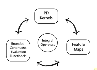
<span class="mw-page-title-main">Reproducing kernel Hilbert space</span> In functional analysis, a Hilbert space

In functional analysis, a reproducing kernel Hilbert space (RKHS) is a Hilbert space of functions in which point evaluation is a continuous linear functional. Roughly speaking, this means that if two functions and in the RKHS are close in norm, i.e., is small, then and are also pointwise close, i.e., is small for all . The converse does not need to be true. Informally, this can be shown by looking at the supremum norm: the sequence of functions converges pointwise, but does not converge uniformly i.e. does not converge with respect to the supremum norm.

In functional analysis, a branch of mathematics, it is sometimes possible to generalize the notion of the determinant of a square matrix of finite order (representing a linear transformation from a finite-dimensional vector space to itself) to the infinite-dimensional case of a linear operator S mapping a function space V to itself. The corresponding quantity det(S) is called the functional determinant of S.
<span class="mw-page-title-main">Wigner's theorem</span> Theorem in the mathematical formulation of quantum mechanics

Wigner's theorem, proved by Eugene Wigner in 1931, is a cornerstone of the mathematical formulation of quantum mechanics. The theorem specifies how physical symmetries such as rotations, translations, and CPT transformations are represented on the Hilbert space of states.

In mathematics, a holomorphic vector bundle is a complex vector bundle over a complex manifold X such that the total space E is a complex manifold and the projection map π : EX is holomorphic. Fundamental examples are the holomorphic tangent bundle of a complex manifold, and its dual, the holomorphic cotangent bundle. A holomorphic line bundle is a rank one holomorphic vector bundle.

In cryptography, learning with errors (LWE) is a mathematical problem that is widely used to create secure encryption algorithms. It is based on the idea of representing secret information as a set of equations with errors. In other words, LWE is a way to hide the value of a secret by introducing noise to it. In more technical terms, it refers to the computational problem of inferring a linear -ary function over a finite ring from given samples some of which may be erroneous. The LWE problem is conjectured to be hard to solve, and thus to be useful in cryptography.

<span class="mw-page-title-main">Wrapped Cauchy distribution</span>

In probability theory and directional statistics, a wrapped Cauchy distribution is a wrapped probability distribution that results from the "wrapping" of the Cauchy distribution around the unit circle. The Cauchy distribution is sometimes known as a Lorentzian distribution, and the wrapped Cauchy distribution may sometimes be referred to as a wrapped Lorentzian distribution.

In mathematics, the Witten zeta function, is a function associated to a root system that encodes the degrees of the irreducible representations of the corresponding Lie group. These zeta functions were introduced by Don Zagier who named them after Edward Witten's study of their special values. Note that in, Witten zeta functions do not appear as explicit objects in their own right.

Least-squares support-vector machines (LS-SVM) for statistics and in statistical modeling, are least-squares versions of support-vector machines (SVM), which are a set of related supervised learning methods that analyze data and recognize patterns, and which are used for classification and regression analysis. In this version one finds the solution by solving a set of linear equations instead of a convex quadratic programming (QP) problem for classical SVMs. Least-squares SVM classifiers were proposed by Johan Suykens and Joos Vandewalle. LS-SVMs are a class of kernel-based learning methods.

Coherent states have been introduced in a physical context, first as quasi-classical states in quantum mechanics, then as the backbone of quantum optics and they are described in that spirit in the article Coherent states. However, they have generated a huge variety of generalizations, which have led to a tremendous amount of literature in mathematical physics. In this article, we sketch the main directions of research on this line. For further details, we refer to several existing surveys.

In algebra and number theory, a distribution is a function on a system of finite sets into an abelian group which is analogous to an integral: it is thus the algebraic analogue of a distribution in the sense of generalised function.

Regularized least squares (RLS) is a family of methods for solving the least-squares problem while using regularization to further constrain the resulting solution.

References

  1. 1 2 Moody, John (1989). "Fast learning in multi-resolution hierarchies" (PDF). Advances in Neural Information Processing Systems.
  2. 1 2 3 4 5 6 7 Kilian Weinberger; Anirban Dasgupta; John Langford; Alex Smola; Josh Attenberg (2009). Feature Hashing for Large Scale Multitask Learning (PDF). Proc. ICML.
  3. 1 2 K. Ganchev; M. Dredze (2008). Small statistical models by random feature mixing (PDF). Proc. ACL08 HLT Workshop on Mobile Language Processing.
  4. Josh Attenberg; Kilian Weinberger; Alex Smola; Anirban Dasgupta; Martin Zinkevich (2009). "Collaborative spam filtering with the hashing trick". Virus Bulletin.
  5. Bai, B.; Weston J.; Grangier D.; Collobert R.; Sadamasa K.; Qi Y.; Chapelle O.; Weinberger K. (2009). Supervised semantic indexing (PDF). CIKM. pp. 187–196.
  6. Chen, Wenlin; Wilson, James; Tyree, Stephen; Weinberger, Kilian; Chen, Yixin (2015-06-01). "Compressing Neural Networks with the Hashing Trick". International Conference on Machine Learning. PMLR: 2285–2294. arXiv: 1504.04788 .
  7. Owen, Sean; Anil, Robin; Dunning, Ted; Friedman, Ellen (2012). Mahout in Action. Manning. pp. 261–265.
  8. "gensim: corpora.hashdictionary – Construct word<->id mappings". Radimrehurek.com. Retrieved 2014-02-13.
  9. "4.1. Feature extraction — scikit-learn 0.14 documentation". Scikit-learn.org. Retrieved 2014-02-13.
  10. "sofia-ml - Suite of Fast Incremental Algorithms for Machine Learning. Includes methods for learning classification and ranking models, using Pegasos SVM, SGD-SVM, ROMMA, Passive-Aggressive Perceptron, Perceptron with Margins, and Logistic Regression" . Retrieved 2014-02-13.
  11. "Hashing TF" . Retrieved 4 September 2015. Maps a sequence of terms to their term frequencies using the hashing trick.
  12. "FeatureHashing: Creates a Model Matrix via Feature Hashing With a Formula Interface". 10 January 2024.
  13. "tf.keras.preprocessing.text.hashing_trick — TensorFlow Core v2.0.1" . Retrieved 2020-04-29. Converts a text to a sequence of indexes in a fixed-size hashing space.
  14. "dask_ml.feature_extraction.text.HashingVectorizer — dask-ml 2021.11.17 documentation". ml.dask.org. Retrieved 2021-11-22.