Kabsch algorithm

Last updated November 12, 2024

The Kabsch algorithm, also known as the Kabsch-Umeyama algorithm,^[1] named after Wolfgang Kabsch and Shinji Umeyama, is a method for calculating the optimal rotation matrix that minimizes the RMSD (root mean squared deviation) between two paired sets of points. It is useful for point-set registration in computer graphics, and in cheminformatics and bioinformatics to compare molecular and protein structures (in particular, see root-mean-square deviation (bioinformatics)).

Description

Let $P$ and $Q$ be two sets, each containing $N$ points in $\mathbb {R} ^{n}$ . We want to find the transformation from $Q$ to $P$ . For simplicity, we will consider the three-dimensional case ( $n=3$ ). The sets $P$ and $Q$ can each be represented by $N \times 3$ matrices with the first row containing the coordinates of the first point, the second row containing the coordinates of the second point, and so on, as shown in this matrix:

${\begin{pmatrix}x_{1}&y_{1}&z_{1}\\x_{2}&y_{2}&z_{2}\\\vdots &\vdots &\vdots \\x_{N}&y_{N}&z_{N}\end{pmatrix}}$

The algorithm works in three steps: a translation, the computation of a covariance matrix, and the computation of the optimal rotation matrix.

Translation

Both sets of coordinates must be translated first, so that their centroid coincides with the origin of the coordinate system. This is done by subtracting the centroid coordinates from the point coordinates.

Computation of the covariance matrix

The second step consists of calculating a matrix $H$ . In matrix notation,

H=P^{\mathsf {T}}Q\,

or, using summation notation,

H_{ij}=\sum _{k=1}^{N}P_{ki}Q_{kj},

which is a cross-covariance matrix when $P$ and $Q$ are seen as data matrices.

Computation of the optimal rotation matrix

It is possible to calculate the optimal rotation $R$ based on the matrix formula

R=\left(H^{\mathsf {T}}H\right)^{\frac {1}{2}}H^{-1},

but implementing a numerical solution to this formula becomes complicated when all special cases are accounted for (for example, the case of $H$ not having an inverse).

If singular value decomposition (SVD) routines are available the optimal rotation, $R$ , can be calculated using the following algorithm.

First, calculate the SVD of the covariance matrix $H$ ,

H=U\Sigma V^{\mathsf {T}}

where $U$ and $V$ are orthogonal and $\Sigma$ is diagonal. Next, record if the orthogonal matrices contain a reflection,

d=\det \left(UV^{\mathsf {T}}\right)=\det(U)\det(V).

Finally, calculate our optimal rotation matrix $R$ as

R=U{\begin{pmatrix}1&0&0\\0&1&0\\0&0&d\end{pmatrix}}V^{\mathsf {T}}.

This $R$ minimizes $\sum _{k=1}^{N}|Rq_{k}-p_{k}|$ , where $q_{k}$ and $p_{k}$ are rows in $Q$ and $P$ respectively.

Alternatively, optimal rotation matrix can also be directly evaluated as quaternion.^[2]^[3]^[4]^[5] This alternative description has been used in the development of a rigorous method for removing rigid-body motions from molecular dynamics trajectories of flexible molecules.^[6] In 2002 a generalization for the application to probability distributions (continuous or not) was also proposed.^[7]

Generalizations

The algorithm was described for points in a three-dimensional space. The generalization to $D$ dimensions is immediate.

External links

This SVD algorithm is described in more detail at https://web.archive.org/web/20140225050055/http://cnx.org/content/m11608/latest/

A Matlab function is available at http://www.mathworks.com/matlabcentral/fileexchange/25746-kabsch-algorithm

A C++ implementation (and unit test) using Eigen

A Python script is available at https://github.com/charnley/rmsd. Another implementation can be found in SciPy.

A free PyMol plugin easily implementing Kabsch is . (This previously linked to CEalign , but this uses the Combinatorial Extension (CE) algorithm.) VMD uses the Kabsch algorithm for its alignment.

The FoldX modeling toolsuite incorporates the Kabsch algorithm to measure RMSD between Wild Type and Mutated protein structures.

Related Research Articles

In mathematical physics and mathematics, the Pauli matrices are a set of three $2 \times 2$ complex matrices that are traceless, Hermitian, involutory and unitary. Usually indicated by the Greek letter sigma, they are occasionally denoted by tau when used in connection with isospin symmetries.

In linear algebra, an orthogonal matrix, or orthonormal matrix, is a real square matrix whose columns and rows are orthonormal vectors.

In mathematics, specifically in linear algebra, matrix multiplication is a binary operation that produces a matrix from two matrices. For matrix multiplication, the number of columns in the first matrix must be equal to the number of rows in the second matrix. The resulting matrix, known as the matrix product, has the number of rows of the first and the number of columns of the second matrix. The product of matrices $A$ and $B$ is denoted as $AB$ .

In mechanics and geometry, the 3D rotation group, often denoted SO(3), is the group of all rotations about the origin of three-dimensional Euclidean space $under the operation of composition.$

Unit quaternions, known as versors, provide a convenient mathematical notation for representing spatial orientations and rotations of elements in three dimensional space. Specifically, they encode information about an axis-angle rotation about an arbitrary axis. Rotation and orientation quaternions have applications in computer graphics, computer vision, robotics, navigation, molecular dynamics, flight dynamics, orbital mechanics of satellites, and crystallographic texture analysis.

In mathematics, the matrix representation of conic sections permits the tools of linear algebra to be used in the study of conic sections. It provides easy ways to calculate a conic section's axis, vertices, tangents and the pole and polar relationship between points and lines of the plane determined by the conic. The technique does not require putting the equation of a conic section into a standard form, thus making it easier to investigate those conic sections whose axes are not parallel to the coordinate system.

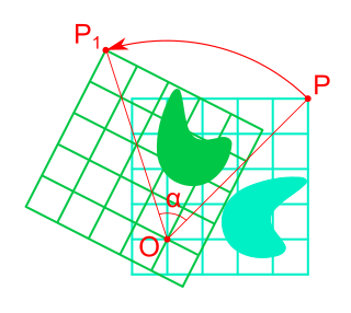
Rotation in mathematics is a concept originating in geometry. Any rotation is a motion of a certain space that preserves at least one point. It can describe, for example, the motion of a rigid body around a fixed point. Rotation can have a sign (as in the sign of an angle): a clockwise rotation is a negative magnitude so a counterclockwise turn has a positive magnitude. A rotation is different from other types of motions: translations, which have no fixed points, and (hyperplane) reflections, each of them having an entire $(n - 1)$ -dimensional flat of fixed points in a $n$ -dimensional space.

In linear algebra, a rotation matrix is a transformation matrix that is used to perform a rotation in Euclidean space. For example, using the convention below, the matrix

In geometry, Euler's rotation theorem states that, in three-dimensional space, any displacement of a rigid body such that a point on the rigid body remains fixed, is equivalent to a single rotation about some axis that runs through the fixed point. It also means that the composition of two rotations is also a rotation. Therefore the set of rotations has a group structure, known as a rotation group.

In mathematics, the Cayley transform, named after Arthur Cayley, is any of a cluster of related things. As originally described by Cayley (1846), the Cayley transform is a mapping between skew-symmetric matrices and special orthogonal matrices. The transform is a homography used in real analysis, complex analysis, and quaternionic analysis. In the theory of Hilbert spaces, the Cayley transform is a mapping between linear operators.

In mathematics, the polar decomposition of a square real or complex matrix $is a factorization of the form, where is a unitary matrix and is a positive semi-definite Hermitian matrix, both square and of the same size.$

In geometry and linear algebra, a Cartesian tensor uses an orthonormal basis to represent a tensor in a Euclidean space in the form of components. Converting a tensor's components from one such basis to another is done through an orthogonal transformation.

In mathematics, the group of rotations about a fixed point in four-dimensional Euclidean space is denoted SO(4). The name comes from the fact that it is the special orthogonal group of order 4.

In statistics, Procrustes analysis is a form of statistical shape analysis used to analyse the distribution of a set of shapes. The name Procrustes refers to a bandit from Greek mythology who made his victims fit his bed either by stretching their limbs or cutting them off.

In bioinformatics, the root mean square deviation of atomic positions, or simply root mean square deviation (RMSD), is the measure of the average distance between the atoms (usually the backbone atoms) of superimposed molecules. In the study of globular protein conformations, one customarily measures the similarity in three-dimensional structure by the RMSD of the Cα atomic coordinates after optimal rigid body superposition.

In computer vision, the essential matrix is a $matrix, that relates corresponding points in stereo images assuming that the cameras satisfy the pinhole camera model.$

<span class="mw-page-title-main">Dual quaternion</span> Eight-dimensional algebra over the real numbers

In mathematics, the dual quaternions are an 8-dimensional real algebra isomorphic to the tensor product of the quaternions and the dual numbers. Thus, they may be constructed in the same way as the quaternions, except using dual numbers instead of real numbers as coefficients. A dual quaternion can be represented in the form A + εB, where A and B are ordinary quaternions and ε is the dual unit, which satisfies ε² = 0 and commutes with every element of the algebra. Unlike quaternions, the dual quaternions do not form a division algebra.

The orthogonal Procrustes problem is a matrix approximation problem in linear algebra. In its classical form, one is given two matrices $and and asked to find an orthogonal matrix which most closely maps to . Specifically, the orthogonal Procrustes problem is an optimization problem given by$

In applied mathematics, Wahba's problem, first posed by Grace Wahba in 1965, seeks to find a rotation matrix between two coordinate systems from a set of (weighted) vector observations. Solutions to Wahba's problem are often used in satellite attitude determination utilising sensors such as magnetometers and multi-antenna GPS receivers. The cost function that Wahba's problem seeks to minimise is as follows:

In mathematics and mechanics, the Euler–Rodrigues formula describes the rotation of a vector in three dimensions. It is based on Rodrigues' rotation formula, but uses a different parametrization.

References

↑ Lawrence, Jim; Bernal, Javier; Witzgall, Christoph (2019-10-09). "A Purely Algebraic Justification of the Kabsch-Umeyama Algorithm" (PDF). Journal of Research of the National Institute of Standards and Technology. 124: 124028. doi:10.6028/jres.124.028. ISSN 2165-7254. PMC 7340555 . PMID 34877177.
↑ Horn, Berthold K. P. (1987-04-01). "Closed-form solution of absolute orientation using unit quaternions". Journal of the Optical Society of America A. 4 (4): 629. Bibcode:1987JOSAA...4..629H. CiteSeerX 10.1.1.68.7320 . doi:10.1364/josaa.4.000629. ISSN 1520-8532. S2CID 11038004.
↑ Kneller, Gerald R. (1991-05-01). "Superposition of Molecular Structures using Quaternions". Molecular Simulation. 7 (1–2): 113–119. doi:10.1080/08927029108022453. ISSN 0892-7022.
↑ Coutsias, E. A.; Seok, C.; Dill, K. A. (2004). "Using quaternions to calculate RMSD". J. Comput. Chem. 25 (15): 1849–1857. doi:10.1002/jcc.20110. PMID 15376254. S2CID 18224579.
↑ Petitjean, M. (1999). "On the root mean square quantitative chirality and quantitative symmetry measures" (PDF). J. Math. Phys. 40 (9): 4587–4595. Bibcode:1999JMP....40.4587P. doi:10.1063/1.532988.
↑ Chevrot, Guillaume; Calligari, Paolo; Hinsen, Konrad; Kneller, Gerald R. (2011-08-24). "Least constraint approach to the extraction of internal motions from molecular dynamics trajectories of flexible macromolecules". J. Chem. Phys. 135 (8): 084110. Bibcode:2011JChPh.135h4110C. doi:10.1063/1.3626275. ISSN 0021-9606. PMID 21895162.
↑ Petitjean, M. (2002). "Chiral mixtures" (PDF). J. Math. Phys. 43 (8): 4147–4157. Bibcode:2002JMP....43.4147P. doi:10.1063/1.1484559. S2CID 85454709.

Kabsch, Wolfgang (1976). "A solution for the best rotation to relate two sets of vectors". Acta Crystallographica. A32 (5): 922. Bibcode:1976AcCrA..32..922K. doi:10.1107/S0567739476001873.
- With a correction in Kabsch, Wolfgang (1978). "A discussion of the solution for the best rotation to relate two sets of vectors". Acta Crystallographica. A34 (5): 827–828. Bibcode:1978AcCrA..34..827K. doi: 10.1107/S0567739478001680 .
Lin, Ying-Hung; Chang, Hsun-Chang; Lin, Yaw-Ling (December 15–17, 2004). A Study on Tools and Algorithms for 3-D Protein Structures Alignment and Comparison. International Computer Symposium. Taipei, Taiwan.
Umeyama, Shinji (1991). "Least-Squares Estimation of Transformation Parameters Between Two Point Patterns". IEEE Trans. Pattern Anal. Mach. Intell. 13 (4): 376–380. doi:10.1109/34.88573.

This page is based on this Wikipedia article
Text is available under the CC BY-SA 4.0 license; additional terms may apply.
Images, videos and audio are available under their respective licenses.

[1] Lawrence, Jim; Bernal, Javier; Witzgall, Christoph (2019-10-09). "A Purely Algebraic Justification of the Kabsch-Umeyama Algorithm" (PDF). Journal of Research of the National Institute of Standards and Technology. 124: 124028. doi:10.6028/jres.124.028. ISSN 2165-7254. PMC 7340555 . PMID 34877177.

[2] Horn, Berthold K. P. (1987-04-01). "Closed-form solution of absolute orientation using unit quaternions". Journal of the Optical Society of America A. 4 (4): 629. Bibcode:1987JOSAA...4..629H. CiteSeerX 10.1.1.68.7320 . doi:10.1364/josaa.4.000629. ISSN 1520-8532. S2CID 11038004.

[3] Kneller, Gerald R. (1991-05-01). "Superposition of Molecular Structures using Quaternions". Molecular Simulation. 7 (1–2): 113–119. doi:10.1080/08927029108022453. ISSN 0892-7022.

[Coutsias2004-4] Coutsias, E. A.; Seok, C.; Dill, K. A. (2004). "Using quaternions to calculate RMSD". J. Comput. Chem. 25 (15): 1849–1857. doi:10.1002/jcc.20110. PMID 15376254. S2CID 18224579.

[Petitjean1999-5] Petitjean, M. (1999). "On the root mean square quantitative chirality and quantitative symmetry measures" (PDF). J. Math. Phys. 40 (9): 4587–4595. Bibcode:1999JMP....40.4587P. doi:10.1063/1.532988.

[6] Chevrot, Guillaume; Calligari, Paolo; Hinsen, Konrad; Kneller, Gerald R. (2011-08-24). "Least constraint approach to the extraction of internal motions from molecular dynamics trajectories of flexible macromolecules". J. Chem. Phys. 135 (8): 084110. Bibcode:2011JChPh.135h4110C. doi:10.1063/1.3626275. ISSN 0021-9606. PMID 21895162.

[Petitjean2002-7] Petitjean, M. (2002). "Chiral mixtures" (PDF). J. Math. Phys. 43 (8): 4147–4157. Bibcode:2002JMP....43.4147P. doi:10.1063/1.1484559. S2CID 85454709.

[1]

[2]

[3]

[4]

[5]

[6]

[7]