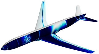
The Navier–Stokes equations are partial differential equations which describe the motion of viscous fluid substances. They were named after French engineer and physicist Claude-Louis Navier and the Irish physicist and mathematician George Gabriel Stokes. They were developed over several decades of progressively building the theories, from 1822 (Navier) to 1842–1850 (Stokes).
In thermal fluid dynamics, the Nusselt number is the ratio of total heat transfer to conductive heat transfer at a boundary in a fluid. Total heat transfer combines conduction and convection. Convection includes both advection and diffusion (conduction). The conductive component is measured under the same conditions as the convective but for a hypothetically motionless fluid. It is a dimensionless number, closely related to the fluid's Rayleigh number.

In fluid dynamics, turbulence or turbulent flow is fluid motion characterized by chaotic changes in pressure and flow velocity. It is in contrast to laminar flow, which occurs when a fluid flows in parallel layers with no disruption between those layers.

In physics and fluid mechanics, a boundary layer is the thin layer of fluid in the immediate vicinity of a bounding surface formed by the fluid flowing along the surface. The fluid's interaction with the wall induces a no-slip boundary condition. The flow velocity then monotonically increases above the surface until it returns to the bulk flow velocity. The thin layer consisting of fluid whose velocity has not yet returned to the bulk flow velocity is called the velocity boundary layer.
The Richardson number (Ri) is named after Lewis Fry Richardson (1881–1953). It is the dimensionless number that expresses the ratio of the buoyancy term to the flow shear term:

In thermodynamics, the Onsager reciprocal relations express the equality of certain ratios between flows and forces in thermodynamic systems out of equilibrium, but where a notion of local equilibrium exists.

The surface layer is the layer of a turbulent fluid most affected by interaction with a solid surface or the surface separating a gas and a liquid where the characteristics of the turbulence depend on distance from the interface. Surface layers are characterized by large normal gradients of tangential velocity and large concentration gradients of any substances transported to or from the interface.

Large eddy simulation (LES) is a mathematical model for turbulence used in computational fluid dynamics. It was initially proposed in 1963 by Joseph Smagorinsky to simulate atmospheric air currents, and first explored by Deardorff (1970). LES is currently applied in a wide variety of engineering applications, including combustion, acoustics, and simulations of the atmospheric boundary layer.
In fluid dynamics, the Reynolds stress is the component of the total stress tensor in a fluid obtained from the averaging operation over the Navier–Stokes equations to account for turbulent fluctuations in fluid momentum.

In fluid dynamics, turbulence modeling is the construction and use of a mathematical model to predict the effects of turbulence. Turbulent flows are commonplace in most real-life scenarios. In spite of decades of research, there is no analytical theory to predict the evolution of these turbulent flows. The equations governing turbulent flows can only be solved directly for simple cases of flow. For most real-life turbulent flows, CFD simulations use turbulent models to predict the evolution of turbulence. These turbulence models are simplified constitutive equations that predict the statistical evolution of turbulent flows.
In physics and fluid mechanics, a Blasius boundary layer describes the steady two-dimensional laminar boundary layer that forms on a semi-infinite plate which is held parallel to a constant unidirectional flow. Falkner and Skan later generalized Blasius' solution to wedge flow, i.e. flows in which the plate is not parallel to the flow.
In fluid dynamics, turbulence kinetic energy (TKE) is the mean kinetic energy per unit mass associated with eddies in turbulent flow. Physically, the turbulence kinetic energy is characterized by measured root-mean-square (RMS) velocity fluctuations. In the Reynolds-averaged Navier Stokes equations, the turbulence kinetic energy can be calculated based on the closure method, i.e. a turbulence model.

In fluid dynamics, eddy diffusion, eddy dispersion, or turbulent diffusion is a process by which fluid substances mix together due to eddy motion. These eddies can vary widely in size, from subtropical ocean gyres down to the small Kolmogorov microscales, and occur as a result of turbulence. The theory of eddy diffusion was first developed by Sir Geoffrey Ingram Taylor.
The derivation of the Navier–Stokes equations as well as their application and formulation for different families of fluids, is an important exercise in fluid dynamics with applications in mechanical engineering, physics, chemistry, heat transfer, and electrical engineering. A proof explaining the properties and bounds of the equations, such as Navier–Stokes existence and smoothness, is one of the important unsolved problems in mathematics.
The turbulent Prandtl number (Prt) is a non-dimensional term defined as the ratio between the momentum eddy diffusivity and the heat transfer eddy diffusivity. It is useful for solving the heat transfer problem of turbulent boundary layer flows. The simplest model for Prt is the Reynolds analogy, which yields a turbulent Prandtl number of 1. From experimental data, Prt has an average value of 0.85, but ranges from 0.7 to 0.9 depending on the Prandtl number of the fluid in question.

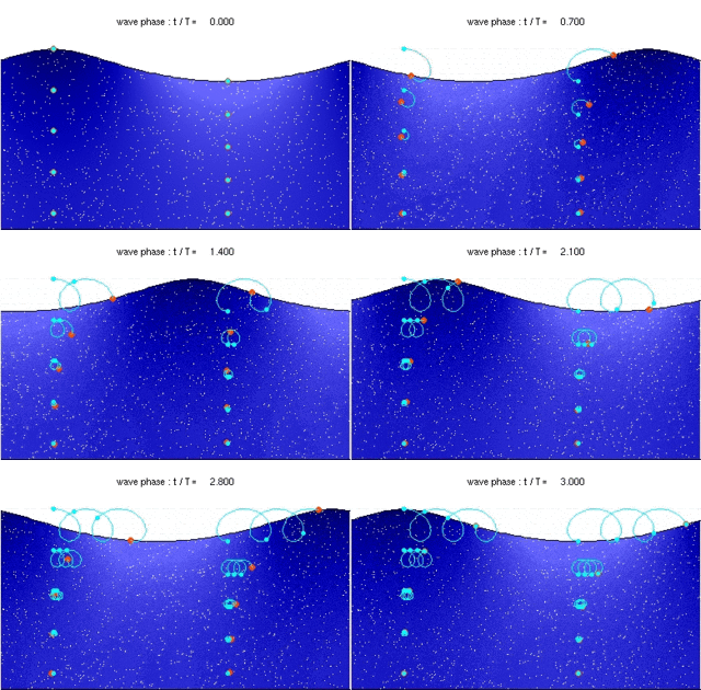
For a pure wave motion in fluid dynamics, the Stokes drift velocity is the average velocity when following a specific fluid parcel as it travels with the fluid flow. For instance, a particle floating at the free surface of water waves, experiences a net Stokes drift velocity in the direction of wave propagation.

In fluid dynamics, the Reynolds number is a dimensionless quantity that helps predict fluid flow patterns in different situations by measuring the ratio between inertial and viscous forces. At low Reynolds numbers, flows tend to be dominated by laminar (sheet-like) flow, while at high Reynolds numbers, flows tend to be turbulent. The turbulence results from differences in the fluid's speed and direction, which may sometimes intersect or even move counter to the overall direction of the flow. These eddy currents begin to churn the flow, using up energy in the process, which for liquids increases the chances of cavitation.

In fluid dynamics, the radiation stress is the depth-integrated – and thereafter phase-averaged – excess momentum flux caused by the presence of the surface gravity waves, which is exerted on the mean flow. The radiation stresses behave as a second-order tensor.
Reynolds stress equation model (RSM), also referred to as second moment closures are the most complete classical turbulence model. In these models, the eddy-viscosity hypothesis is avoided and the individual components of the Reynolds stress tensor are directly computed. These models use the exact Reynolds stress transport equation for their formulation. They account for the directional effects of the Reynolds stresses and the complex interactions in turbulent flows. Reynolds stress models offer significantly better accuracy than eddy-viscosity based turbulence models, while being computationally cheaper than Direct Numerical Simulations (DNS) and Large Eddy Simulations.
Monin–Obukhov (M–O) similarity theory describes the non-dimensionalized mean flow and mean temperature in the surface layer under non-neutral conditions as a function of the dimensionless height parameter, named after Russian scientists A. S. Monin and A. M. Obukhov. Similarity theory is an empirical method that describes universal relationships between non-dimensionalized variables of fluids based on the Buckingham π theorem. Similarity theory is extensively used in boundary layer meteorology since relations in turbulent processes are not always resolvable from first principles.


