Mode choice analysis is the third step in the conventional four-step transportation forecasting model of transportation planning, following trip distribution and preceding route assignment. From origin-destination table inputs provided by trip distribution, mode choice analysis allows the modeler to determine probabilities that travelers will use a certain mode of transport. These probabilities are called the modal share, and can be used to produce an estimate of the amount of trips taken using each feasible mode.
The early transportation planning model developed by the Chicago Area Transportation Study (CATS) focused on transit. It wanted to know how much travel would continue by transit. The CATS divided transit trips into two classes: trips to the Central Business District, or CBD (mainly by subway/elevated transit, express buses, and commuter trains) and other (mainly on the local bus system). For the latter, increases in auto ownership and use were a trade-off against bus use; trend data were used. CBD travel was analyzed using historic mode choice data together with projections of CBD land uses. Somewhat similar techniques were used in many studies. Two decades after CATS, for example, the London study followed essentially the same procedure, but in this case, researchers first divided trips into those made in the inner part of the city and those in the outer part. This procedure was followed because it was thought that income (resulting in the purchase and use of automobiles) drove mode choice.
Diversion curve techniques
The CATS had diversion curve techniques available and used them for some tasks. At first, the CATS studied the diversion of auto traffic from streets and arterial roads to proposed expressways. Diversion curves were also used for bypasses built around cities to find out what percent of traffic would use the bypass. The mode choice version of diversion curve analysis proceeds this way: one forms a ratio, say:
where:
cm = travel time by mode m and
R is empirical data in the form:
Figure: Mode choice diversion curve
Given the R that we have calculated, the graph tells us the percent of users in the market that will choose transit. A variation on the technique is to use costs rather than time in the diversion ratio. The decision to use a time or cost ratio turns on the problem at hand. Transit agencies developed diversion curves for different kinds of situations, so variables like income and population density entered implicitly.
Diversion curves are based on empirical observations, and their improvement has resulted from better (more and more pointed) data. Curves are available for many markets. It is not difficult to obtain data and array results. Expansion of transit has motivated data development by operators and planners. Yacov Zahavi’s UMOT studies, discussed earlier, contain many examples of diversion curves.
In a sense, diversion curve analysis is expert system analysis. Planners could "eyeball" neighborhoods and estimate transit ridership by routes and time of day. Instead, diversion is observed empirically and charts drawn.
Disaggregate travel demand models
Travel demand theory was introduced in the appendix on traffic generation. The core of the field is the set of models developed following work by Stan Warner in 1962 (Strategic Choice of Mode in Urban Travel: A Study of Binary Choice). Using data from the CATS, Warner investigated classification techniques using models from biology and psychology. Building from Warner and other early investigators, disaggregate demand models emerged. Analysis is disaggregate in that individuals are the basic units of observation, yet aggregate because models yield a single set of parameters describing the choice behavior of the population. Behavior enters because the theory made use of consumer behavior concepts from economics and parts of choice behavior concepts from psychology. Researchers at the University of California, Berkeley (especially Daniel McFadden, who won a Nobel Prize in Economics for his efforts) and the Massachusetts Institute of Technology (Moshe Ben-Akiva) (and in MIT associated consulting firms, especially Cambridge Systematics) developed what has become known as choice models, direct demand models (DDM), Random Utility Models (RUM) or, in its most used form, the multinomial logit model (MNL).
Choice models have attracted a lot of attention and work; the Proceedings of the International Association for Travel Behavior Research chronicles the evolution of the models. The models are treated in modern transportation planning and transportation engineering textbooks.
One reason for rapid model development was a felt need. Systems were being proposed (especially transit systems) where no empirical experience of the type used in diversion curves was available. Choice models permit comparison of more than two alternatives and the importance of attributes of alternatives. There was the general desire for an analysis technique that depended less on aggregate analysis and with a greater behavioral content. And there was attraction, too, because choice models have logical and behavioral roots extended back to the 1920s as well as roots in Kelvin Lancaster’s consumer behavior theory, in utility theory, and in modern statistical methods.
Psychological roots
Distribution of perceived weights
Early psychology work involved the typical experiment: Here are two objects with weights, w1 and w2, which is heavier? The finding from such an experiment would be that the greater the difference in weight, the greater the probability of choosing correctly. Graphs similar to the one on the right result.
The assumption that e is normally and identically distributed (NID) yields the binary probit model.
Econometric formulation
Economists deal with utility rather than physical weights, and say that
observed utility = mean utility + random term.
The characteristics of the object, x, must be considered, so we have
u(x) = v(x) + e(x).
If we follow Thurston's assumption, we again have a probit model.
An alternative is to assume that the error terms are independently and identically distributed with a Weibull, Gumbel Type I, or double exponential distribution. (They are much the same, and differ slightly in their tails (thicker) from the normal distribution). This yields the multinomial logit model (MNL). Daniel McFadden argued that the Weibull had desirable properties compared to other distributions that might be used. Among other things, the error terms are normally and identically distributed. The logit model is simply a log ratio of the probability of choosing a mode to the probability of not choosing a mode.
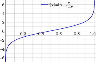
Observe the mathematical similarity between the logit model and the S-curves we estimated earlier, although here share increases with utility rather than time. With a choice model we are explaining the share of travelers using a mode (or the probability that an individual traveler uses a mode multiplied by the number of travelers).
The comparison with S-curves is suggestive that modes (or technologies) get adopted as their utility increases, which happens over time for several reasons. First, because the utility itself is a function of network effects, the more users, the more valuable the service, higher the utility associated with joining the network. Second because utility increases as user costs drop, which happens when fixed costs can be spread over more users (another network effect). Third technological advances, which occur over time and as the number of users increases, drive down relative cost.
An illustration of a utility expression is given:
where
Pi = Probability of choosing mode i.
PA = Probability of taking auto
cA,cT = cost of auto, transit
tA,tT = travel time of auto, transit
I = income
N = Number of travelers
With algebra, the model can be translated to its most widely used form:
It is fair to make two conflicting statements about the estimation and use of this model:
it's a "house of cards", and
used by a technically competent and thoughtful analyst, it's useful.
The "house of cards" problem largely arises from the utility theory basis of the model specification. Broadly, utility theory assumes that (1) users and suppliers have perfect information about the market; (2) they have deterministic functions (faced with the same options, they will always make the same choices); and (3) switching between alternatives is costless. These assumptions don’t fit very well with what is known about behavior. Furthermore, the aggregation of utility across the population is impossible since there is no universal utility scale.
Suppose an option has a net utility ujk (option k, person j). We can imagine that having a systematic part vjk that is a function of the characteristics of an object and person j, plus a random part ejk, which represents tastes, observational errors and a bunch of other things (it gets murky here). (An object such as a vehicle does not have utility, it is characteristics of a vehicle that have utility.) The introduction of e lets us do some aggregation. As noted above, we think of observable utility as being a function:
where each variable represents a characteristic of the auto trip. The value β0 is termed an alternative specific constant. Most modelers say it represents characteristics left out of the equation (e.g., the political correctness of a mode, if I take transit I feel morally righteous, so β0 may be negative for the automobile), but it includes whatever is needed to make error terms NID.
Econometric estimation
Figure: Likelihood Function for the Sample {1,1,1,0,1}.
Turning now to some technical matters, how do we estimate v(x)? Utility (v(x)) isn’t observable. All we can observe are choices (say, measured as 0 or 1), and we want to talk about probabilities of choices that range from 0 to 1. (If we do a regression on 0s and 1s we might measure for j a probability of 1.4 or −0.2 of taking an auto.) Further, the distribution of the error terms wouldn’t have appropriate statistical characteristics.
The MNL approach is to make a maximum likelihood estimate of this functional form. The likelihood function is:
we solve for the estimated parameters
that maxL*. This happens when:
The log-likelihood is easier to work with, as the products turn to sums:
Consider an example adopted from John Bitzan’s Transportation Economics Notes. Let X be a binary variable that is equal to 1 with probability γ, and equal to 0 with probability (1−gamma). Then f(0) = (1−γ) and f(1) = γ. Suppose that we have 5 observations of X, giving the sample {1,1,1,0,1}. To find the maximum likelihood estimator of γ examine various values of γ, and for these values determine the probability of drawing the sample {1,1,1,0,1} If γ takes the value 0, the probability of drawing our sample is 0. If γ is 0.1, then the probability of getting our sample is: f(1,1,1,0,1) = f(1)f(1)f(1)f(0)f(1) = 0.1×0.1×0.1×0.9×0.1 = 0.00009 We can compute the probability of obtaining our sample over a range of γ – this is our likelihood function. The likelihood function for n independent observations in a logit model is
where: Yi = 1 or 0 (choosing e.g. auto or not-auto) and Pi = the probability of observing Yi=1
The log likelihood is thus:
In the binomial (two alternative) logit model,
, so
The log-likelihood function is maximized setting the partial derivatives to zero:
The above gives the essence of modern MNL choice modeling.
Additional topics
Topics not touched on include the “red bus, blue bus” problem; the use of nested models (e.g., estimate choice between auto and transit, and then estimate choice between rail and bus transit); how consumers’ surplus measurements may be obtained; and model estimation, goodness of fit, etc. For these topics see a textbook such as Ortuzar and Willumsen (2001).
Returning to roots
The discussion above is based on the economist’s utility formulation. At the time MNL modeling was developed there was some attention to psychologist's choice work (e.g., Luce’s choice axioms discussed in his Individual Choice Behavior, 1959). It has an analytic side in computational process modeling. Emphasis is on how people think when they make choices or solve problems (see Newell and Simon 1972). Put another way, in contrast to utility theory, it stresses not the choice but the way the choice was made. It provides a conceptual framework for travel choices and agendas of activities involving considerations of long and short term memory, effectors, and other aspects of thought and decision processes. It takes the form of rules dealing with the way information is searched and acted on. Although there is a lot of attention to behavioral analysis in transportation work, the best of modern psychological ideas are only beginning to enter the field. (e.g. Golledge, Kwan and Garling 1984; Garling, Kwan, and Golledge 1994).
External links
Transportation Systems Analysis Model – TSAM is a nationwide transportation planning model to forecast intercity travel behavior in the United States.
In statistics, the logit function is the quantile function associated with the standard logistic distribution. It has many uses in data analysis and machine learning, especially in data transformations.
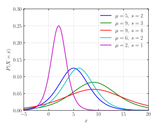
In probability theory and statistics, the beta distribution is a family of continuous probability distributions defined on the interval [0, 1] parameterized by two positive shape parameters, denoted by alpha (α) and beta (β), that appear as exponents of the random variable and control the shape of the distribution. The generalization to multiple variables is called a Dirichlet distribution.
In statistics, the logistic model is a statistical model that models the probability of an event taking place by having the log-odds for the event be a linear combination of one or more independent variables. In regression analysis, logistic regression is estimating the parameters of a logistic model. Formally, in binary logistic regression there is a single binary dependent variable, coded by an indicator variable, where the two values are labeled "0" and "1", while the independent variables can each be a binary variable or a continuous variable. The corresponding probability of the value labeled "1" can vary between 0 and 1, hence the labeling; the function that converts log-odds to probability is the logistic function, hence the name. The unit of measurement for the log-odds scale is called a logit, from logistic unit, hence the alternative names. See § Background and § Definition for formal mathematics, and § Example for a worked example.
In probability theory and statistics, the Gumbel distribution is used to model the distribution of the maximum of a number of samples of various distributions.
In probability theory and statistics, the logistic distribution is a continuous probability distribution. Its cumulative distribution function is the logistic function, which appears in logistic regression and feedforward neural networks. It resembles the normal distribution in shape but has heavier tails. The logistic distribution is a special case of the Tukey lambda distribution.
In statistics, a generalized linear model (GLM) is a flexible generalization of ordinary linear regression. The GLM generalizes linear regression by allowing the linear model to be related to the response variable via a link function and by allowing the magnitude of the variance of each measurement to be a function of its predicted value.
Trip distribution is the second component in the traditional four-step transportation forecasting model. This step matches tripmakers’ origins and destinations to develop a “trip table”, a matrix that displays the number of trips going from each origin to each destination. Historically, this component has been the least developed component of the transportation planning model.
In probability theory and statistics, the generalized extreme value (GEV) distribution is a family of continuous probability distributions developed within extreme value theory to combine the Gumbel, Fréchet and Weibull families also known as type I, II and III extreme value distributions. By the extreme value theorem the GEV distribution is the only possible limit distribution of properly normalized maxima of a sequence of independent and identically distributed random variables. Note that a limit distribution needs to exist, which requires regularity conditions on the tail of the distribution. Despite this, the GEV distribution is often used as an approximation to model the maxima of long (finite) sequences of random variables.
In statistics, a probit model is a type of regression where the dependent variable can take only two values, for example married or not married. The word is a portmanteau, coming from probability + unit. The purpose of the model is to estimate the probability that an observation with particular characteristics will fall into a specific one of the categories; moreover, classifying observations based on their predicted probabilities is a type of binary classification model.
In information theory, the cross-entropy between two probability distributions and over the same underlying set of events measures the average number of bits needed to identify an event drawn from the set if a coding scheme used for the set is optimized for an estimated probability distribution , rather than the true distribution .
In statistics, multinomial logistic regression is a classification method that generalizes logistic regression to multiclass problems, i.e. with more than two possible discrete outcomes. That is, it is a model that is used to predict the probabilities of the different possible outcomes of a categorically distributed dependent variable, given a set of independent variables.
In statistics, semiparametric regression includes regression models that combine parametric and nonparametric models. They are often used in situations where the fully nonparametric model may not perform well or when the researcher wants to use a parametric model but the functional form with respect to a subset of the regressors or the density of the errors is not known. Semiparametric regression models are a particular type of semiparametric modelling and, since semiparametric models contain a parametric component, they rely on parametric assumptions and may be misspecified and inconsistent, just like a fully parametric model.
In economics, discrete choice models, or qualitative choice models, describe, explain, and predict choices between two or more discrete alternatives, such as entering or not entering the labor market, or choosing between modes of transport. Such choices contrast with standard consumption models in which the quantity of each good consumed is assumed to be a continuous variable. In the continuous case, calculus methods can be used to determine the optimum amount chosen, and demand can be modeled empirically using regression analysis. On the other hand, discrete choice analysis examines situations in which the potential outcomes are discrete, such that the optimum is not characterized by standard first-order conditions. Thus, instead of examining "how much" as in problems with continuous choice variables, discrete choice analysis examines "which one". However, discrete choice analysis can also be used to examine the chosen quantity when only a few distinct quantities must be chosen from, such as the number of vehicles a household chooses to own and the number of minutes of telecommunications service a customer decides to purchase. Techniques such as logistic regression and probit regression can be used for empirical analysis of discrete choice.
In statistics, binomial regression is a regression analysis technique in which the response has a binomial distribution: it is the number of successes in a series of independent Bernoulli trials, where each trial has probability of success . In binomial regression, the probability of a success is related to explanatory variables: the corresponding concept in ordinary regression is to relate the mean value of the unobserved response to explanatory variables.
Mixed logit is a fully general statistical model for examining discrete choices. It overcomes three important limitations of the standard logit model by allowing for random taste variation across choosers, unrestricted substitution patterns across choices, and correlation in unobserved factors over time. Mixed logit can choose any distribution for the random coefficients, unlike probit which is limited to the normal distribution. It is called "mixed logit" because the choice probability is a mixture of logits, with as the mixing distribution. It has been shown that a mixed logit model can approximate to any degree of accuracy any true random utility model of discrete choice, given appropriate specification of variables and the coefficient distribution.
Although the concept choice models is widely understood and practiced these days, it is often difficult to acquire hands-on knowledge in simulating choice models. While many stat packages provide useful tools to simulate, researchers attempting to test and simulate new choice models with data often encounter problems from as simple as scaling parameter to misspecification. This article goes beyond simply defining discrete choice models. Rather, it aims at providing a comprehensive overview of how to simulate such models in computer.
In probability theory and statistics, the Exponential-Logarithmic (EL) distribution is a family of lifetime distributions with decreasing failure rate, defined on the interval [0, ∞). This distribution is parameterized by two parameters and .
In statistics and econometrics, the maximum score estimator is a nonparametric estimator for discrete choice models developed by Charles Manski in 1975. Unlike the multinomial probit and multinomial logit estimators, it makes no assumptions about the distribution of the unobservable part of utility. However, its statistical properties are more complicated than the multinomial probit and logit models, making statistical inference difficult. To address these issues, Joel Horowitz proposed a variant, called the smoothed maximum score estimator.
Ordinal data is a categorical, statistical data type where the variables have natural, ordered categories and the distances between the categories are not known. These data exist on an ordinal scale, one of four levels of measurement described by S. S. Stevens in 1946. The ordinal scale is distinguished from the nominal scale by having a ranking. It also differs from the interval scale and ratio scale by not having category widths that represent equal increments of the underlying attribute.
The hyperbolastic functions, also known as hyperbolastic growth models, are mathematical functions that are used in medical statistical modeling. These models were originally developed to capture the growth dynamics of multicellular tumor spheres, and were introduced in 2005 by Mohammad Tabatabai, David Williams, and Zoran Bursac. The precision of hyperbolastic functions in modeling real world problems is somewhat due to their flexibility in their point of inflection. These functions can be used in a wide variety of modeling problems such as tumor growth, stem cell proliferation, pharma kinetics, cancer growth, sigmoid activation function in neural networks, and epidemiological disease progression or regression.
References
Garling, Tommy, Mei-Po Kwan, and Reginald G. Golledge. Household Activity Scheduling, Transportation Research, 22B, pp.333–353. 1994.
Golledge. Reginald G., Mei Po Kwan, and Tommy Garling, “Computational Process Modeling of Household Travel Decisions,” Papers in Regional Science, 73, pp.99–118. 1984.
Lancaster, K.J., A new approach to consumer theory. Journal of Political Economy, 1966. 74(2): p.132–157.
Luce, Duncan R. (1959). Individual choice behavior, a theoretical analysis. New York, Wiley.
Newell, A. and Simon, H. A. (1972). Human Problem Solving. Englewood Cliffs, NJ: Prentice Hall.
Ortuzar, Juan de Dios and L. G. Willumsen’s Modelling Transport. 3rd Edition. Wiley and Sons. 2001,
Thurstone, L.L. (1927). A law of comparative judgement. Psychological Review, 34, 278–286.
Warner, Stan 1962 Strategic Choice of Mode in Urban Travel: A Study of Binary Choice
This page is based on this Wikipedia article Text is available under the CC BY-SA 4.0 license; additional terms may apply. Images, videos and audio are available under their respective licenses.