P system

Last updated
For the computer p-System, see UCSD p-System.

A P system is a computational model in the field of computer science that performs calculations using a biologically inspired process. They are based upon the structure of biological cells, abstracting from the way in which chemicals interact and cross cell membranes. The concept was first introduced in a 1998 report [1] by the computer scientist Gheorghe Păun, whose last name is the origin of the letter P in 'P Systems'. Variations on the P system model led to the formation of a branch of research known as 'membrane computing.'

Contents

Although inspired by biology, the primary research interest in P systems is concerned with their use as a computational model, rather than for biological modeling, [2] although this is also being investigated. [3] [4] [5]

Informal description

A P system is defined as a series of membranes containing chemicals (in finite quantities), catalysts and rules which determine possible ways in which chemicals may react with one another to form products. Rules may also cause chemicals to pass through membranes or even cause membranes to dissolve.

Just as in a biological cell, where a chemical reaction may only take place upon the chance event that the required chemical molecules collide and interact (possibly also with a catalyst), the rules in a P system are applied at random. This causes the computation to proceed in a non-deterministic manner, often resulting in multiple solutions being encountered if the computation is repeated.

A P system continues until it reaches a state where no further reactions are possible. At this point the result of the computation is all those chemicals that have been passed outside of the outermost membrane, or otherwise those passed into a designated 'result' membrane. [4]

Components of a P system

Although many varieties of P system exist, most share the same basic components. Each element has a specific role to play, and each has a founding in the biological cell architecture upon which P systems are based.

The environment

The environment is the surroundings of the P system. In the initial state of a P system it contains only the container-membrane, and while the environment can never hold rules, it may have objects passed into it during the computation. The objects found within the environment at the end of the computation constitute all or part of its “result.”

Membranes

Membranes are the main “structures” within a P system. A membrane is a discrete unit which can contain a set of objects (symbols/catalysts), a set of rules, and a set of other membranes contained within. The outermost membrane, held within the environment, is often referred to as the 'container membrane' or 'skin membrane'. As implied to by their namesake, membranes are permeable and symbols resulting from a rule may cross them. A membrane (but not the container membrane) may also “dissolve”, in which case its content, except for rules (which are lost), migrate into the membrane in which it was contained. [2]

Some P system variants allow for a membrane to divide, possess a charge or have varying permeability by changing membrane thickness. [2]

Symbols

Symbols represent chemicals that may react with other chemicals to form some product. In a P system, each type of symbol is typically represented by a different letter. The symbol content of a membrane is therefore represented by a string of letters. Because the multiplicity of symbols in a region matters, multisets are commonly used to represent the symbol content of a region.

Special case symbols exist, for example, a lower case delta (δ) is often used to initiate the dissolving of a membrane, and this will only ever be found in the output of a rule: upon being encountered it invokes a reaction, and is used in the process.

Catalysts

Catalysts are similar to their namesakes in chemistry. They are represented and used in the same way as symbols, but are never consumed during a “reaction,” they are simply a requirement for it to occur.

Rules

Rules represent a possible chemical reaction within a membrane, causing it to evolve to a new state. A rule has a required set of input objects (symbols or catalysts) that must be present in order for it to be applied. If the required objects are present, it consumes them and produces a set of output objects. A rule may also be specified to have a priority over other rules, in which case less dominant rules will only be applied when it is not possible to apply a more dominant rule (i.e. the required inputs are not present).

There are three (in the basic P system model) distinct ways in which a rule may handle its output objects. Usually, the output objects are passed into the current membrane (the same membrane in which the rule and the inputs reside), known as a here rule. However, there are two modifiers that can be specified upon output objects when rules are defined, in and out. The in modifier causes the object to be passed to one of the current membrane's children (travelling inwards relative to the structure of the P system), chosen at random during the computation. The out modifier causes the object to be passed out of the current membrane and into either its parent membrane or to a sibling membrane, specified during specification of the P system.

Computation process

A computation works from an initial starting state towards an end state through a number of discrete steps. Each step involves iterating through all membranes in the P system and the application of rules, which occurs in both a maximally parallel and non-deterministic manner. [4]

Working through step-by-step, a computation halts when no further evolution can take place (i.e. when no rules are able to be applied). At this point whatever objects have been passed to the environment, or into a designated 'result' membrane, are counted as the result of the computation. [4]

Rule application

At each step of a computation an object may only be used once, as they are consumed by rules when applied. The method of applying a rule within a membrane is as follows:

  1. Assign symbols from a membrane's content to the rule's inputs
  2. If all inputs are satisfied, remove all assigned symbols from membrane
  3. Create output symbols and hold until all rule assignment, for all membranes, has taken place.
  4. Add output symbols to targeted membranes.
  5. Dissolve membranes as necessary

Outputs are not passed immediately into membranes because this would contravene the maximally parallel nature of rule application, instead they are distributed after all possible rules have been applied.

Non-deterministic application

The order of rule application is chosen at random. Rule application order can have a significant effect on which rules may be applied at any given time, and the outcome of a step of execution.

Consider a membrane containing only a single "a" symbol, and the two rules a → ab and a → aδ. As both rules rely on an “a” symbol being present, of which there is only one, the first step of computation will allow either the first or second rule to be applied, but not both. The two possible results of this step are very different:

  1. The membrane carries over to the next step of the computation with both an "a" symbol and a "b" symbol present, and again one of the two rules is randomly assigned to the "a" symbol.
  2. The membrane dissolves and a single "a" symbol is passed out to the containing membrane.

Maximally parallel application

This is a property of rule application whereby all possible rule assignments must take place during every step of the computation. In essence this means that the rule a → aa has the effect of doubling the number of "a" symbols in its containing membrane each step, because the rule is applied to every occurrence of an "a" symbol present.

As a computational model

Most P systems variants are computationally universal. [4] This extends even to include variants that do not use rule priorities, usually a fundamental aspect of P systems. [6]

As a model for computation, P systems offer the attractive possibility of solving NP-complete problems in less-than exponential time. [4] Some P system variants are known to be capable of solving the SAT (boolean satisfiability) problem in linear time [7] and, owing to all NP-complete problems being equivalent, this capability then applies to all such problems. As there is no current method of directly implementing a P system in its own right, their functionality is instead emulated [8] and therefore solving NP-complete problems in linear time remains theoretical. However, it has also been proven that any deterministic P system may be simulated on a Turing Machine in polynomial time. [2]

Example computation

The graphical representation of a P system which outputs square numbers P-system-example.svg
The graphical representation of a P system which outputs square numbers

The image shown depicts the initial state of a P system with three membranes. Because of their hierarchical nature, P systems are often depicted graphically with drawings that resemble Venn diagrams or David Harel's Higraph (see Statechart).

The outermost membrane, 1, is the container membrane for this P system and contains a single out rule. Membrane 2 contains four here rules, with two in a priority relationship: cc → c will always be applied in preference to c → δ. The delta symbol represents the special “dissolve” symbol. The innermost membrane, 3, contains a set of symbols (“ac”) and three rules, of type here. In this initial state no rules outside of membrane 3 are applicable: there are no symbols outside of that membrane. However, during evolution of the system, as objects are passed between membranes, the rules in other membranes will become active.

Computation

Because of the non-deterministic nature of P systems, there are many different paths of computation a single P system is capable of, leading to different results. The following is one possible path of computation for the P system depicted.

Step 1

From the initial configuration only membrane 3 has any object content: "ac"

  • "c" is assigned to c → cc
  • "a" is assigned to a → ab

Step 2

Membrane 3 now contains: "abcc"

  • "a" is assigned to a → bδ
  • "c" is assigned to c → cc
  • "c" is assigned to c → cc

Notice the maximally parallel behaviour of rule application leading to the same rule being applied twice during one step.

Notice also that the application of the second rule (a → bδ) as opposed to the first (a → ab) is non-deterministic and can be presumed random. The system could just as well have continued applying the first rule (and at the same time doubling the c particles) indefinitely.

Membrane 3 now dissolves, as the dissolve symbol (δ) has been encountered and all object content from this membrane passes into membrane 2.

Step 3

Membrane 2 now contains: "bbcccc"

  • "b" is assigned to b → d
  • "b" is assigned to b → d
  • "cc" is assigned to cc → c
  • "cc" is assigned to cc → c

Step 4

Membrane 2 now contains: "ddcc"

  • "d" is assigned to d → de
  • "d" is assigned to d → de
  • "cc" is assigned to cc → c

Step 5

Membrane 2 now contains: "dedec"

  • "d" is assigned to d → de
  • "d" is assigned to d → de
  • "c" is assigned to c → δ

Notice that the priority over c → δ has been lifted now the required inputs for cc→ c no longer exist. Membrane 2 now dissolves, and all object content passes to membrane 1.

Step 6

Membrane 1 now contains: "deedee"

  • "e” is assigned to e → eout
  • "e” is assigned to e → eout
  • "e” is assigned to e → eout
  • "e” is assigned to e → eout

Computation halts

Membrane 1 now contains: "dd" and, due to the out rule e → eout, the environment contains: "eeee." At this point the computation halts as no further assignments of objects to rules is possible. The result of the computation is four "e" symbols.

The only non-deterministic choices occurred during steps 1 and 2, when choosing where to assign the solitary "a" symbol. Consider the case where "a" is assigned to a → bδ during step 1: upon membrane 3 dissolving only a single "b" and two "c" objects would exist, leading to the creation of only a single "e" object to eventually be passed out as the computation's result.

See also

Related Research Articles

<span class="mw-page-title-main">Finite-state machine</span> Mathematical model of computation

A finite-state machine (FSM) or finite-state automaton, finite automaton, or simply a state machine, is a mathematical model of computation. It is an abstract machine that can be in exactly one of a finite number of states at any given time. The FSM can change from one state to another in response to some inputs; the change from one state to another is called a transition. An FSM is defined by a list of its states, its initial state, and the inputs that trigger each transition. Finite-state machines are of two types—deterministic finite-state machines and non-deterministic finite-state machines. For any non-deterministic finite-state machine, an equivalent deterministic one can be constructed.

In theoretical computer science, a nondeterministic Turing machine (NTM) is a theoretical model of computation whose governing rules specify more than one possible action when in some given situations. That is, an NTM's next state is not completely determined by its action and the current symbol it sees, unlike a deterministic Turing machine.

<span class="mw-page-title-main">Pushdown automaton</span> Type of automaton

In the theory of computation, a branch of theoretical computer science, a pushdown automaton (PDA) is a type of automaton that employs a stack.

<span class="mw-page-title-main">Turing machine</span> Computation model defining an abstract machine

A Turing machine is a mathematical model of computation describing an abstract machine that manipulates symbols on a strip of tape according to a table of rules. Despite the model's simplicity, it is capable of implementing any computer algorithm.

In computer science, an abstract machine is a theoretical model that allows for a detailed and precise analysis of how a computer system functions. It is similar to a mathematical function in that it receives inputs and produces outputs based on predefined rules. Abstract machines vary from literal machines in that they are expected to perform correctly and independently of hardware. Abstract machines are "machines" because they allow step-by-step execution of programmes; they are "abstract" because they ignore many aspects of actual (hardware) machines. A typical abstract machine consists of a definition in terms of input, output, and the set of allowable operations used to turn the former into the latter. They can be used for purely theoretical reasons as well as models for real-world computer systems. In the theory of computation, abstract machines are often used in thought experiments regarding computability or to analyse the complexity of algorithms. This use of abstract machines is fundamental to the field of computational complexity theory, such as finite state machines, Mealy machines, push-down automata, and Turing machines.

<span class="mw-page-title-main">Automata theory</span> Study of abstract machines and automata

Automata theory is the study of abstract machines and automata, as well as the computational problems that can be solved using them. It is a theory in theoretical computer science with close connections to mathematical logic. The word automata comes from the Greek word αὐτόματος, which means "self-acting, self-willed, self-moving". An automaton is an abstract self-propelled computing device which follows a predetermined sequence of operations automatically. An automaton with a finite number of states is called a Finite Automaton (FA) or Finite-State Machine (FSM). The figure on the right illustrates a finite-state machine, which is a well-known type of automaton. This automaton consists of states and transitions. As the automaton sees a symbol of input, it makes a transition to another state, according to its transition function, which takes the previous state and current input symbol as its arguments.

<span class="mw-page-title-main">State diagram</span> Diagram of behavior of finite state systems

A state diagram is a type of diagram used in computer science and related fields to describe the behavior of systems. State diagrams require that the system is composed of a finite number of states. Sometimes, this is indeed the case, while at other times this is a reasonable abstraction. Many forms of state diagrams exist, which differ slightly and have different semantics.

In the theory of computation, a tag system is a deterministic model of computation published by Emil Leon Post in 1943 as a simple form of a Post canonical system. A tag system may also be viewed as an abstract machine, called a Post tag machine —briefly, a finite-state machine whose only tape is a FIFO queue of unbounded length, such that in each transition the machine reads the symbol at the head of the queue, deletes a constant number of symbols from the head, and appends to the tail a symbol-string that depends solely on the first symbol read in this transition.

<span class="mw-page-title-main">Deterministic finite automaton</span> Finite-state machine

In the theory of computation, a branch of theoretical computer science, a deterministic finite automaton (DFA)—also known as deterministic finite acceptor (DFA), deterministic finite-state machine (DFSM), or deterministic finite-state automaton (DFSA)—is a finite-state machine that accepts or rejects a given string of symbols, by running through a state sequence uniquely determined by the string. Deterministic refers to the uniqueness of the computation run. In search of the simplest models to capture finite-state machines, Warren McCulloch and Walter Pitts were among the first researchers to introduce a concept similar to finite automata in 1943.

In automata theory, a finite-state machine is called a deterministic finite automaton (DFA), if

In computational complexity theory, an alternating Turing machine (ATM) is a non-deterministic Turing machine (NTM) with a rule for accepting computations that generalizes the rules used in the definition of the complexity classes NP and co-NP. The concept of an ATM was set forth by Chandra and Stockmeyer and independently by Kozen in 1976, with a joint journal publication in 1981.

The X-machine (XM) is a theoretical model of computation introduced by Samuel Eilenberg in 1974. The X in "X-machine" represents the fundamental data type on which the machine operates; for example, a machine that operates on databases would be a database-machine. The X-machine model is structurally the same as the finite-state machine, except that the symbols used to label the machine's transitions denote relations of type XX. Crossing a transition is equivalent to applying the relation that labels it, and traversing a path in the machine corresponds to applying all the associated relations, one after the other.

<span class="mw-page-title-main">Kahn process networks</span> Model of computation

A Kahn process network is a distributed model of computation in which a group of deterministic sequential processes communicate through unbounded first in, first out channels. The model requires that reading from a channel is blocking while writing is non-blocking. Due to these key restrictions, the resulting process network exhibits deterministic behavior that does not depend on the timing of computation nor on communication delays.

Unconventional computing is computing by any of a wide range of new or unusual methods. It is also known as alternative computing.

A Turing machine is a hypothetical computing device, first conceived by Alan Turing in 1936. Turing machines manipulate symbols on a potentially infinite strip of tape according to a finite table of rules, and they provide the theoretical underpinnings for the notion of a computer algorithm.

<span class="mw-page-title-main">Membrane computing</span>

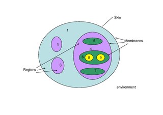
Membrane computing is an area within computer science that seeks to discover new computational models from the study of biological cells, particularly of the cellular membranes. It is a sub-task of creating a cellular model.

Membrane systems have been inspired from the structure and the functioning of the living cells. They were introduced and studied by Gh.Paun under the name of P systems [24]; some applications of the membrane systems are presented in [15]. Membrane systems are essentially models of distributed, parallel and nondeterministic systems. Here we motivate and present the mobile membranes. Mobile membranes represent a variant of membrane systems inspired by the biological movements given by endocytosis and exocytosis. They have the expressive power of both P systems and process calculi with mobility such as mobile ambients [11] and brane calculi [10]. Computations with mobile membranes can be defined over specific configurations, while they represent also a rule-based formalism.

Natural computing, also called natural computation, is a terminology introduced to encompass three classes of methods: 1) those that take inspiration from nature for the development of novel problem-solving techniques; 2) those that are based on the use of computers to synthesize natural phenomena; and 3) those that employ natural materials to compute. The main fields of research that compose these three branches are artificial neural networks, evolutionary algorithms, swarm intelligence, artificial immune systems, fractal geometry, artificial life, DNA computing, and quantum computing, among others.

In computational learning theory, induction of regular languages refers to the task of learning a formal description of a regular language from a given set of example strings. Although E. Mark Gold has shown that not every regular language can be learned this way, approaches have been investigated for a variety of subclasses. They are sketched in this article. For learning of more general grammars, see Grammar induction.

In theoretical computer science, in particular in formal language theory, Kleene's algorithm transforms a given nondeterministic finite automaton (NFA) into a regular expression. Together with other conversion algorithms, it establishes the equivalence of several description formats for regular languages. Alternative presentations of the same method include the "elimination method" attributed to Brzozowski and McCluskey, the algorithm of McNaughton and Yamada, and the use of Arden's lemma.

References

  1. Păun, Gheorghe (1998). Computing with Membranes. TUCS Report 208. Turku Centre for Computer Science. ISBN   978-952-12-0303-9 . Retrieved 16 December 2012.
  2. 1 2 3 4 Păun, Gheorghe; Grzegorz Rozenberg (2002). "A guide to membrane computing". Theoretical Computer Science. 287 (1): 73–100. CiteSeerX   10.1.1.76.8425 . doi:10.1016/S0304-3975(02)00136-6. ISSN   0304-3975.
  3. Ardelean, Ioan; Matteo Cavaliere (June 2003). "Modelling biological processes by using a probabilistic p system software". Natural Computing. 2 (2): 173–197. doi:10.1023/A:1024943605864. ISSN   1567-7818.
  4. 1 2 3 4 5 6 Păun, Gheorghe (2006). "Introduction to Membrane Computing". Applications of Membrane Computing. Springer Berlin Heidelberg. pp. 1–42. ISBN   978-3-540-29937-0.
  5. Nash, Anthony; Sara Kalvala (2019). "A P system model of swarming and aggregation in a Myxobacterial colony". Journal of Membrane Computing. 1: 103–11. doi: 10.1007/s41965-019-00015-0 .
  6. Freund, Rudolf; Kari, Lila; Oswald, Marion; Sosík, Petr (2005). "Computationally universal P systems without priorities: two catalysts are sufficient". Theoretical Computer Science. 330 (2): 251–266. doi:10.1016/j.tcs.2004.06.029. ISSN   0304-3975.
  7. Păun, Gheorghe (2001). "P systems with active membranes: attacking NP-complete problems" (PDF). Automata, Languages and Combinatorics. 6 (1): 75–90. Retrieved 2008-02-03.
  8. Zandron, Claudio; Claudio Ferretti; Giancarlo Mauri (2000). "Solving NP-Complete Problems Using P Systems with Active Membranes". Unconventional Models of Computation. pp. 289–301. ISBN   1-85233-415-0.