Significance arithmetic

Last updated

Significance arithmetic is a set of rules (sometimes called significant figure rules) for approximating the propagation of uncertainty in scientific or statistical calculations. These rules can be used to find the appropriate number of significant figures to use to represent the result of a calculation. If a calculation is done without analysis of the uncertainty involved, a result that is written with too many significant figures can be taken to imply a higher precision than is known, and a result that is written with too few significant figures results in an avoidable loss of precision. Understanding these rules requires a good understanding of the concept of significant and insignificant figures.

Contents

The rules of significance arithmetic are an approximation based on statistical rules for dealing with probability distributions. See the article on propagation of uncertainty for these more advanced and precise rules. Significance arithmetic rules rely on the assumption that the number of significant figures in the operands gives accurate information about the uncertainty of the operands and hence the uncertainty of the result. For alternatives see Interval arithmetic and Floating-point error mitigation.

An important caveat is that significant figures apply only to measured values. Values known to be exact should be ignored for determining the number of significant figures that belong in the result. Examples of such values include:

Physical constants such as the gravitational constant, however, have a limited number of significant digits, because these constants are known to us only by measurement. On the other hand, c (the speed of light) is exactly 299,792,458 m/s by definition.

Multiplication and division using significance arithmetic

When multiplying or dividing numbers, the result is rounded to the number of significant figures in the factor with the least significant figures. Here, the quantity of significant figures in each of the factors is important—not the position of the significant figures. For instance, using significance arithmetic rules:

If, in the above, the numbers are assumed to be measurements (and therefore probably inexact) then "8" above represents an inexact measurement with only one significant digit. Therefore, the result of "8 × 8" is rounded to a result with only one significant digit, i.e., "6 × 101" instead of the unrounded "64" that one might expect. In many cases, the rounded result is less accurate than the non-rounded result; a measurement of "8" has an actual underlying quantity between 7.5 and 8.5. The true square would be in the range between 56.25 and 72.25. So 6 × 101 is the best one can give, as other possible answers give a false sense of accuracy. Further, the 6 × 101 is itself confusing (as it might be considered to imply 60 ± 5, which is over-optimistic; more accurate would be 64 ± 8).

Addition and subtraction using significance arithmetic

When adding or subtracting using significant figures rules, results are rounded to the position of the least significant digit in the most uncertain of the numbers being added (or subtracted).[ citation needed ] That is, the result is rounded to the last digit that is significant in each of the numbers being summed. Here the position of the significant figures is important, but the quantity of significant figures is irrelevant. Some examples using these rules are:

1
+1.1
2
1.0
+1.1
2.1
9.9
9.9
9.9
9.9
3.3
+1.1
40.0

Transcendental functions

Transcendental functions have a complicated method to determine the significance of the function output. These include logarithmic functions, exponential functions and the trigonometric functions. The significance of the output depends on the condition number. In general, the number of significant figures of the output is equal to the number of significant figures of the function input (function argument) minus the order of magnitude of the condition number.

The condition number of a differentiable function at a point is (see details):

Note that if a function has a zero at a point, its condition number at the point is infinite, as infinitesimal changes in the input can change the output from zero to non-zero, yielding a ratio with zero in the denominator, hence an infinite relative change. The condition number of the most used functions are as follows; [1] these can be used to compute significant figures for all elementary functions:

NameSymbolCondition number
Addition / subtraction
Scalar multiplication
Division
Polynomial
Exponential function
Logarithm with base b
Natural logarithm function
Sine function
Cosine function
Tangent function
Inverse sine function
Inverse cosine function
Inverse tangent function

Derivation

The fact that the number of significant figures of the function output is equal to the number of significant figures of the function input (function argument) minus the base-10 logarithm of the condition number (which is approximately the order of magnitude/number of digits of the condition number) can be easily derived from first principles: let and be the true values and let and be approximate values with errors and respectively, so that

and .

Then

,

and hence

.

The significant figures of a number is related to the uncertain error of the number by

where "significant figures of x" here means the number of significant figures of x. Substituting this into the above equation gives

.

Therefore

giving, finally:

.

Rounding rules

Because significance arithmetic involves rounding, it is useful to understand a specific rounding rule that is often used when doing scientific calculations: the round-to-even rule (also called banker's rounding). It is especially useful when dealing with large data sets.

This rule helps to eliminate the upwards skewing of data when using traditional rounding rules. Whereas traditional rounding always rounds up when the following digit is 5, bankers sometimes round down to eliminate this upwards bias. See the article on rounding for more information on rounding rules and a detailed explanation of the round-to-even rule.

Disagreements about importance

Significant figures are used extensively in high school and undergraduate courses as a shorthand for the precision with which a measurement is known. However, significant figures are not a perfect representation of uncertainty, and are not meant to be. Instead, they are a useful tool for avoiding expressing more information than the experimenter actually knows, and for avoiding rounding numbers in such a way as to lose precision.

For example, here are some important differences between significant figure rules and uncertainty:

In order to explicitly express the uncertainty in any uncertain result, the uncertainty should be given separately, with an uncertainty interval, and a confidence interval. The expression 1.23 U95 = 0.06 implies that the true (unknowable) value of the variable is expected to lie in the interval from 1.17 to 1.29 with at least 95% confidence. If the confidence interval is not specified it has traditionally been assumed to be 95% corresponding to two standard deviations from the mean. Confidence intervals at one standard deviation (68%) and three standard deviations (99%) are also commonly used.

See also

Related Research Articles

In number theory, an arithmetic, arithmetical, or number-theoretic function is generally any function f(n) whose domain is the positive integers and whose range is a subset of the complex numbers. Hardy & Wright include in their definition the requirement that an arithmetical function "expresses some arithmetical property of n". There is a larger class of number-theoretic functions that do not fit this definition, for example, the prime-counting functions. This article provides links to functions of both classes.

In calculus, the chain rule is a formula that expresses the derivative of the composition of two differentiable functions f and g in terms of the derivatives of f and g. More precisely, if is the function such that for every x, then the chain rule is, in Lagrange's notation,

In numerical analysis, the condition number of a function measures how much the output value of the function can change for a small change in the input argument. This is used to measure how sensitive a function is to changes or errors in the input, and how much error in the output results from an error in the input. Very frequently, one is solving the inverse problem: given one is solving for x, and thus the condition number of the (local) inverse must be used.

<span class="mw-page-title-main">Floating-point arithmetic</span> Computer approximation for real numbers

In computing, floating-point arithmetic (FP) is arithmetic that represents subsets of real numbers using an integer with a fixed precision, called the significand, scaled by an integer exponent of a fixed base. Numbers of this form are called floating-point numbers. For example, 12.345 is a floating-point number in base ten with five digits of precision:

<span class="mw-page-title-main">Dirac delta function</span> Generalized function whose value is zero everywhere except at zero

In mathematical analysis, the Dirac delta function, also known as the unit impulse, is a generalized function on the real numbers, whose value is zero everywhere except at zero, and whose integral over the entire real line is equal to one. Since there is no function having this property, to model the delta "function" rigorously involves the use of limits or, as is common in mathematics, measure theory and the theory of distributions.

A finite difference is a mathematical expression of the form f (x + b) − f (x + a). If a finite difference is divided by ba, one gets a difference quotient. The approximation of derivatives by finite differences plays a central role in finite difference methods for the numerical solution of differential equations, especially boundary value problems.

<span class="mw-page-title-main">Zeeman effect</span> Spectral line splitting in magnetic field

The Zeeman effect is the effect of splitting of a spectral line into several components in the presence of a static magnetic field. It is named after the Dutch physicist Pieter Zeeman, who discovered it in 1896 and received a Nobel prize for this discovery. It is analogous to the Stark effect, the splitting of a spectral line into several components in the presence of an electric field. Also similar to the Stark effect, transitions between different components have, in general, different intensities, with some being entirely forbidden, as governed by the selection rules.

<span class="mw-page-title-main">Riemann sum</span> Approximation technique in integral calculus

In mathematics, a Riemann sum is a certain kind of approximation of an integral by a finite sum. It is named after nineteenth century German mathematician Bernhard Riemann. One very common application is in numerical integration, i.e., approximating the area of functions or lines on a graph, where it is also known as the rectangle rule. It can also be applied for approximating the length of curves and other approximations.

In vector calculus, Green's theorem relates a line integral around a simple closed curve C to a double integral over the plane region D bounded by C. It is the two-dimensional special case of Stokes' theorem.

<span class="mw-page-title-main">Product rule</span> Formula for the derivative of a product

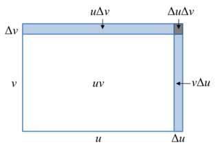
In calculus, the product rule is a formula used to find the derivatives of products of two or more functions. For two functions, it may be stated in Lagrange's notation as

In physics, an operator is a function over a space of physical states onto another space of physical states. The simplest example of the utility of operators is the study of symmetry. Because of this, they are useful tools in classical mechanics. Operators are even more important in quantum mechanics, where they form an intrinsic part of the formulation of the theory.

In the calculus of variations, a field of mathematical analysis, the functional derivative relates a change in a functional to a change in a function on which the functional depends.

<span class="mw-page-title-main">Quantization (signal processing)</span> Process of mapping a continuous set to a countable set

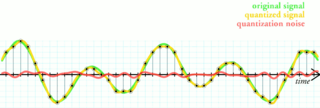
Quantization, in mathematics and digital signal processing, is the process of mapping input values from a large set to output values in a (countable) smaller set, often with a finite number of elements. Rounding and truncation are typical examples of quantization processes. Quantization is involved to some degree in nearly all digital signal processing, as the process of representing a signal in digital form ordinarily involves rounding. Quantization also forms the core of essentially all lossy compression algorithms.

Significant figures, also referred to as significant digits or sig figs, are specific digits within a number written in positional notation that carry both reliability and necessity in conveying a particular quantity. When presenting the outcome of a measurement, if the number of digits exceeds what the measurement instrument can resolve, only the number of digits within the resolution's capability are dependable and therefore considered significant.

A directional derivative is a concept in multivariable calculus that measures the rate at which a function changes in a particular direction at a given point.

In quantum mechanics, the canonical commutation relation is the fundamental relation between canonical conjugate quantities. For example,

In mathematics, the total derivative of a function f at a point is the best linear approximation near this point of the function with respect to its arguments. Unlike partial derivatives, the total derivative approximates the function with respect to all of its arguments, not just a single one. In many situations, this is the same as considering all partial derivatives simultaneously. The term "total derivative" is primarily used when f is a function of several variables, because when f is a function of a single variable, the total derivative is the same as the ordinary derivative of the function.

<span class="mw-page-title-main">Flory–Huggins solution theory</span> Lattice model of polymer solutions

Flory–Huggins solution theory is a lattice model of the thermodynamics of polymer solutions which takes account of the great dissimilarity in molecular sizes in adapting the usual expression for the entropy of mixing. The result is an equation for the Gibbs free energy change for mixing a polymer with a solvent. Although it makes simplifying assumptions, it generates useful results for interpreting experiments.

In calculus, the differential represents the principal part of the change in a function with respect to changes in the independent variable. The differential is defined by

<span class="mw-page-title-main">Envelope (waves)</span> Smooth curve outlining the extremes of an oscillating signal

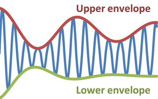
In physics and engineering, the envelope of an oscillating signal is a smooth curve outlining its extremes. The envelope thus generalizes the concept of a constant amplitude into an instantaneous amplitude. The figure illustrates a modulated sine wave varying between an upper envelope and a lower envelope. The envelope function may be a function of time, space, angle, or indeed of any variable.

References

  1. Harrison, John (June 2009). "Decimal Transcendentals via Binary" (PDF). IEEE. Retrieved 2019-12-01.
  2. William Kahan (1 March 1998). "How JAVA's Floating-Point Hurts Everyone Everywhere" (PDF). pp. 37–39.

Further reading