
In mathematics, a spherical coordinate system is a coordinate system for three-dimensional space where the position of a point is specified by three numbers: the radial distance of that point from a fixed origin, its polar angle measured from a fixed zenith direction, and the azimuthal angle of its orthogonal projection on a reference plane that passes through the origin and is orthogonal to the zenith, measured from a fixed reference direction on that plane. It can be seen as the three-dimensional version of the polar coordinate system.

In mathematics and physics, Laplace's equation is a second-order partial differential equation named after Pierre-Simon Laplace who first studied its properties. This is often written as

In physics, the Navier–Stokes equations are a set of partial differential equations which describe the motion of viscous fluid substances, named after French engineer and physicist Claude-Louis Navier and Anglo-Irish physicist and mathematician George Gabriel Stokes.
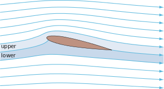
In fluid dynamics, potential flow describes the velocity field as the gradient of a scalar function: the velocity potential. As a result, a potential flow is characterized by an irrotational velocity field, which is a valid approximation for several applications. The irrotationality of a potential flow is due to the curl of the gradient of a scalar always being equal to zero.
In mathematics, the Laplace operator or Laplacian is a differential operator given by the divergence of the gradient of a function on Euclidean space. It is usually denoted by the symbols , , or . In a Cartesian coordinate system, the Laplacian is given by the sum of second partial derivatives of the function with respect to each independent variable. In other coordinate systems, such as cylindrical and spherical coordinates, the Laplacian also has a useful form. Informally, the Laplacian Δf(p) of a function f at a point p measures by how much the average value of f over small spheres or balls centered at p deviates from f(p).
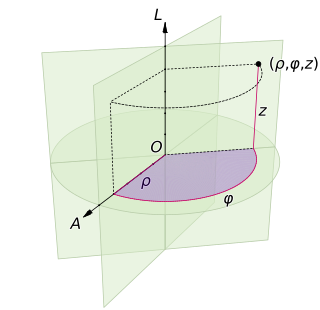
A cylindrical coordinate system is a three-dimensional coordinate system that specifies point positions by the distance from a chosen reference axis, the direction from the axis relative to a chosen reference direction, and the distance from a chosen reference plane perpendicular to the axis. The latter distance is given as a positive or negative number depending on which side of the reference plane faces the point.
In 1851, George Gabriel Stokes derived an expression, now known as Stokes law, for the frictional force – also called drag force – exerted on spherical objects with very small Reynolds numbers in a viscous fluid. Stokes' law is derived by solving the Stokes flow limit for small Reynolds numbers of the Navier–Stokes equations.
The stream function is defined for incompressible (divergence-free) flows in two dimensions – as well as in three dimensions with axisymmetry. The flow velocity components can be expressed as the derivatives of the scalar stream function. The stream function can be used to plot streamlines, which represent the trajectories of particles in a steady flow. The two-dimensional Lagrange stream function was introduced by Joseph Louis Lagrange in 1781. The Stokes stream function is for axisymmetrical three-dimensional flow, and is named after George Gabriel Stokes.

Stokes flow, also named creeping flow or creeping motion, is a type of fluid flow where advective inertial forces are small compared with viscous forces. The Reynolds number is low, i.e. . This is a typical situation in flows where the fluid velocities are very slow, the viscosities are very large, or the length-scales of the flow are very small. Creeping flow was first studied to understand lubrication. In nature this type of flow occurs in the swimming of microorganisms and sperm and the flow of lava. In technology, it occurs in paint, MEMS devices, and in the flow of viscous polymers generally.
In fluid mechanics, potential vorticity (PV) is a quantity which is proportional to the dot product of vorticity and stratification. This quantity, following a parcel of air or water, can only be changed by diabatic or frictional processes. It is a useful concept for understanding the generation of vorticity in cyclogenesis, especially along the polar front, and in analyzing flow in the ocean.
The intent of this article is to highlight the important points of the derivation of the Navier–Stokes equations as well as its application and formulation for different families of fluids.

In fluid dynamics, the Taylor–Green vortex is an unsteady flow of a decaying vortex, which has an exact closed form solution of the incompressible Navier–Stokes equations in Cartesian coordinates. It is named after the British physicist and mathematician Geoffrey Ingram Taylor and his collaborator A. E. Green.
In mathematics, vector spherical harmonics (VSH) are an extension of the scalar spherical harmonics for use with vector fields. The components of the VSH are complex-valued functions expressed in the spherical coordinate basis vectors.
In fluid dynamics, the Oseen equations describe the flow of a viscous and incompressible fluid at small Reynolds numbers, as formulated by Carl Wilhelm Oseen in 1910. Oseen flow is an improved description of these flows, as compared to Stokes flow, with the (partial) inclusion of convective acceleration.

In fluid dynamics, the mild-slope equation describes the combined effects of diffraction and refraction for water waves propagating over bathymetry and due to lateral boundaries—like breakwaters and coastlines. It is an approximate model, deriving its name from being originally developed for wave propagation over mild slopes of the sea floor. The mild-slope equation is often used in coastal engineering to compute the wave-field changes near harbours and coasts.

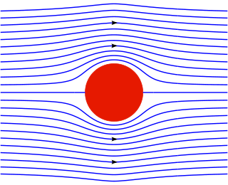
In mathematics, potential flow around a circular cylinder is a classical solution for the flow of an inviscid, incompressible fluid around a cylinder that is transverse to the flow. Far from the cylinder, the flow is unidirectional and uniform. The flow has no vorticity and thus the velocity field is irrotational and can be modeled as a potential flow. Unlike a real fluid, this solution indicates a net zero drag on the body, a result known as d'Alembert's paradox.
In general relativity, the Weyl metrics are a class of static and axisymmetric solutions to Einstein's field equation. Three members in the renowned Kerr–Newman family solutions, namely the Schwarzschild, nonextremal Reissner–Nordström and extremal Reissner–Nordström metrics, can be identified as Weyl-type metrics.
Conformastatic spacetimes refer to a special class of static solutions to Einstein's equation in general relativity.
Elementary flow is a collection of basic flows from which is possible to construct more complex flows by superposition. Some of the flows reflect specific cases and constraints such as incompressible, irrotational or both as in the case of Potential flow.
In fluid dynamics, Hicks equation or sometimes also referred as Bragg–Hawthorne equation or Squire–Long equation is a partial differential equation that describes the distribution of stream function for axisymmetric inviscid fluid, named after William Mitchinson Hicks, who derived it first in 1898. The equation was also re-derived by Stephen Bragg and William Hawthorne in 1950 and by Robert R. Long in 1953 and by Herbert Squire in 1956. The Hicks equation without swirl was first introduced by George Gabriel Stokes in 1842. The Grad–Shafranov equation appearing in plasma physics also takes the same form as the Hicks equation.


