
In statistics, a normal distribution is a type of continuous probability distribution for a real-valued random variable. The general form of its probability density function is

In mathematics, the Dirac delta distribution, also known as the unit impulse symbol, is a generalized function or distribution over the real numbers, whose value is zero everywhere except at zero, and whose integral over the entire real line is equal to one.

Stellar dynamics is the branch of astrophysics which describes in a statistical way the collective motions of stars subject to their mutual gravity. The essential difference from celestial mechanics is that the number of body
In mathematics, the total variation identifies several slightly different concepts, related to the structure of the codomain of a function or a measure. For a real-valued continuous function f, defined on an interval [a, b] ⊂ R, its total variation on the interval of definition is a measure of the one-dimensional arclength of the curve with parametric equation x ↦ f(x), for x ∈ [a, b]. Functions whose total variation is finite are called functions of bounded variation.
In the theory of stochastic processes, the Karhunen–Loève theorem, also known as the Kosambi–Karhunen–Loève theorem is a representation of a stochastic process as an infinite linear combination of orthogonal functions, analogous to a Fourier series representation of a function on a bounded interval. The transformation is also known as Hotelling transform and eigenvector transform, and is closely related to principal component analysis (PCA) technique widely used in image processing and in data analysis in many fields.

In probability theory, a distribution is said to be stable if a linear combination of two independent random variables with this distribution has the same distribution, up to location and scale parameters. A random variable is said to be stable if its distribution is stable. The stable distribution family is also sometimes referred to as the Lévy alpha-stable distribution, after Paul Lévy, the first mathematician to have studied it.
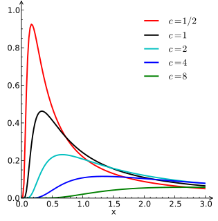
In probability theory and statistics, the Lévy distribution, named after Paul Lévy, is a continuous probability distribution for a non-negative random variable. In spectroscopy, this distribution, with frequency as the dependent variable, is known as a van der Waals profile. It is a special case of the inverse-gamma distribution. It is a stable distribution.

In quantum field theory, the LSZ reduction formula is a method to calculate S-matrix elements from the time-ordered correlation functions of a quantum field theory. It is a step of the path that starts from the Lagrangian of some quantum field theory and leads to prediction of measurable quantities. It is named after the three German physicists Harry Lehmann, Kurt Symanzik and Wolfhart Zimmermann.
In mathematics, the Hankel transform expresses any given function f(r) as the weighted sum of an infinite number of Bessel functions of the first kind Jν(kr). The Bessel functions in the sum are all of the same order ν, but differ in a scaling factor k along the r axis. The necessary coefficient Fν of each Bessel function in the sum, as a function of the scaling factor k constitutes the transformed function. The Hankel transform is an integral transform and was first developed by the mathematician Hermann Hankel. It is also known as the Fourier–Bessel transform. Just as the Fourier transform for an infinite interval is related to the Fourier series over a finite interval, so the Hankel transform over an infinite interval is related to the Fourier–Bessel series over a finite interval.
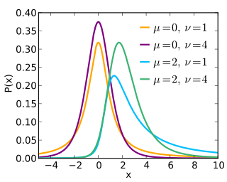
The noncentral t-distribution generalizes Student's t-distribution using a noncentrality parameter. Whereas the central probability distribution describes how a test statistic t is distributed when the difference tested is null, the noncentral distribution describes how t is distributed when the null is false. This leads to its use in statistics, especially calculating statistical power. The noncentral t-distribution is also known as the singly noncentral t-distribution, and in addition to its primary use in statistical inference, is also used in robust modeling for data.
In mathematics and economics, transportation theory or transport theory is a name given to the study of optimal transportation and allocation of resources. The problem was formalized by the French mathematician Gaspard Monge in 1781.
In mathematical analysis, and especially in real, harmonic analysis and functional analysis, an Orlicz space is a type of function space which generalizes the Lp spaces. Like the Lp spaces, they are Banach spaces. The spaces are named for Władysław Orlicz, who was the first to define them in 1932.
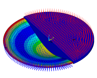
Bending of plates, or plate bending, refers to the deflection of a plate perpendicular to the plane of the plate under the action of external forces and moments. The amount of deflection can be determined by solving the differential equations of an appropriate plate theory. The stresses in the plate can be calculated from these deflections. Once the stresses are known, failure theories can be used to determine whether a plate will fail under a given load.
A product distribution is a probability distribution constructed as the distribution of the product of random variables having two other known distributions. Given two statistically independent random variables X and Y, the distribution of the random variable Z that is formed as the product
In statistics, the generalized Marcum Q-function of order is defined as
Coherent states have been introduced in a physical context, first as quasi-classical states in quantum mechanics, then as the backbone of quantum optics and they are described in that spirit in the article Coherent states. However, they have generated a huge variety of generalizations, which have led to a tremendous amount of literature in mathematical physics. In this article, we sketch the main directions of research on this line. For further details, we refer to several existing surveys.

In mathematics, Ramanujan's master theorem is a technique that provides an analytic expression for the Mellin transform of an analytic function.
Lagrangian field theory is a formalism in classical field theory. It is the field-theoretic analogue of Lagrangian mechanics. Lagrangian mechanics is used to analyze the motion of a system of discrete particles each with a finite number of degrees of freedom. Lagrangian field theory applies to continua and fields, which have an infinite number of degrees of freedom.
In representation theory of mathematics, the Waldspurger formula relates the special values of two L-functions of two related admissible irreducible representations. Let k be the base field, f be an automorphic form over k, π be the representation associated via the Jacquet–Langlands correspondence with f. Goro Shimura (1976) proved this formula, when and f is a cusp form; Günter Harder made the same discovery at the same time in an unpublished paper. Marie-France Vignéras (1980) proved this formula, when and f is a newform. Jean-Loup Waldspurger, for whom the formula is named, reproved and generalized the result of Vignéras in 1985 via a totally different method which was widely used thereafter by mathematicians to prove similar formulas.

In probability theory, the stable count distribution is the conjugate prior of a one-sided stable distribution. This distribution was discovered by Stephen Lihn in his 2017 study of daily distributions of the S&P 500 and the VIX. The stable distribution family is also sometimes referred to as the Lévy alpha-stable distribution, after Paul Lévy, the first mathematician to have studied it.


