Three-phase traffic theory

Three-phase traffic theory is a theory of traffic flow developed by Boris Kerner between 1996 and 2002. ^{[1] [2] [3]} It focuses mainly on the explanation of the physics of traffic breakdown and resulting congested traffic on highways. Kerner describes three phases of traffic, while the classical theories based on the fundamental diagram of traffic flow have two phases: free flow and congested traffic. Kerner’s theory divides congested traffic into two distinct phases, synchronized flow and wide moving jam, bringing the total number of phases to three:

Synchronized flow

Jam

1. Free flow (F)
2. Synchronized flow (S)
3. Wide moving jam (J)

The word "wide" is used even though it is the length of the traffic jam that is being referred to.

A phase is defined as a state in space and time.

Free flow (F)

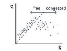
In free traffic flow, empirical data show a positive correlation between the flow rate ${\displaystyle q}$ (in vehicles per unit time) and vehicle density ${\displaystyle k}$ (in vehicles per unit distance). This relationship stops at the maximum free flow ${\displaystyle q_{\max }}$ with a corresponding critical density ${\displaystyle k_{\text{crit}}}$. (See Figure 1.)

Figure 1: Measured flow rate versus vehicle density in free flow (fictitious data)

Congested traffic

Data show a weaker relationship between flow and density in congested conditions. Therefore, Kerner argues that the fundamental diagram, as used in classical traffic theory, cannot adequately describe the complex dynamics of vehicular traffic. He instead divides congestion into synchronized flow and wide moving jams.

In congested traffic, the vehicle speed is lower than the lowest vehicle speed ${\displaystyle v_{\text{free}}^{\min }}$ encountered in free flow, i.e., the line with the slope of the minimal speed ${\displaystyle v_{\text{free}}^{\min }={\frac {q_{\max }}{k_{\text{crit}}}}}$ in free flow (dotted line in Figure 2) divides the empirical data on the flow-density plane into two regions: on the left side data points of free flow and on the right side data points corresponding to congested traffic.

Figure 2: Flow rate versus vehicle density in free flow and congested traffic (fictitious data)

Definitions [J] and [S] of the phases J and S in congested traffic

In Kerner's theory, the phases J and S in congested traffic are observed outcomes in universal spatial-temporal features of real traffic data. The phases J and S are defined through the definitions [J] and [S] as follows:

Figure 3: Measured data of speed in time and space (a) and its representation on the time-space plane (b)

The "wide moving jam" phase [J]

A so-called "wide moving jam" moves upstream through any highway bottlenecks. While doing so, the mean velocity of the downstream front ${\displaystyle v_{g}}$ is maintained. This is the characteristic feature of the wide moving jam that defines the phase J.

The term wide moving jam is meant to reflect the characteristic feature of the jam to propagate through any other state of traffic flow and through any bottleneck while maintaining the velocity of the downstream jam front. The phrase moving jam reflects the jam propagation as a whole localized structure on a road. To distinguish wide moving jams from other moving jams, which do not characteristically maintain the mean velocity of the downstream jam front, Kerner used the term wide. The term wide reflects the fact that if a moving jam has a width (in the longitudinal road direction) considerably greater than the widths of the jam fronts, and if the vehicle speed inside the jam is zero, the jam always exhibits the characteristic feature of maintaining the velocity of the downstream jam front (see Sec. 7.6.5 of the book ^[4] ). Thus the term wide has nothing to do with the width across the jam, but actually refers to its length being considerably more than the transition zones at its head and tail. Historically, Kerner used the term wide from a qualitative analogy of a wide moving jam in traffic flow with wide autosolitons occurring in many systems of natural science (like gas plasma, electron-hole plasma in semiconductors, biological systems, and chemical reactions): Both the wide moving jam and a wide autosoliton exhibit some characteristic features, which do not depend on initial conditions at which these localized patterns have occurred.

The "synchronized flow" phase [S]

In "synchronized flow," the downstream front, where the vehicles accelerate to free flow, does not show this characteristic feature of the wide moving jam. Specifically, the downstream front of the synchronized flow is often fixed at a bottleneck.

The term "synchronized flow" is meant to reflect the following features of this traffic phase: (i) It is a continuous traffic flow with no significant stoppage, as often occurs inside a wide moving jam. The term "flow" reflects this feature. (ii) There is a tendency towards synchronization of vehicle speeds across different lanes on a multilane road in this flow. In addition, there is a tendency towards synchronization of vehicle speeds in each of the road lanes (bunching of vehicles) in synchronized flow. This is due to a relatively low probability of passing. The term "synchronized" reflects this speed synchronization effect.

Explanation of the traffic phase definitions based on measured traffic data

Measured data of averaged vehicle speeds (Figure 3 (a)) illustrate the phase definitions [J] and [S]. There are two spatial-temporal patterns of congested traffic with low vehicle speeds in Figure 3 (a). One pattern propagates upstream with an almost constant velocity of the downstream front, moving straight through the freeway bottleneck. According to the definition [J], this pattern of congestion belongs to the "wide moving jam" phase. In contrast, the downstream front of the other pattern is fixed at a bottleneck. According to the definition [S], this pattern belongs to the "synchronized flow" phase (Figure 3 (a) and (b)). Other empirical examples of the validation of the traffic phase definitions [J] and [S] can be found in the books ^[4] and, ^{[5] [6]} in the article ^[7] as well as in an empirical study of floating car data ^[8] (floating car data is also called probe vehicle data).

Traffic phase definition based on empirical single-vehicle data

In Sec. 6.1 of the book ^[5] has been shown that the traffic phase definitions [S] and [J] are the origin of most hypotheses of three-phase theory and related three-phase microscopic traffic flow models. The traffic phase definitions [J] and [S] are non-local macroscopic ones and they are applicable only after macroscopic data has been measured in space and time, i.e., in an "off-line" study. This is because for the definitive distinction of the phases J and S through the definitions [J] and [S] a study of the propagation of traffic congestion through a bottleneck is necessary. This is often considered as a drawback of the traffic phase definitions [S] and [J]. However, there are local microscopic criteria for the distinction between the phases J and S without a study of the propagation of congested traffic through a bottleneck. The microscopic criteria are as follows (see Sec. 2.6 in the book ^[5] ): If in single-vehicle (microscopic) data related to congested traffic the "flow-interruption interval", i.e., a time headway between two vehicles following each other is observed, which is much longer than the mean time delay in vehicle acceleration from a wide moving jam (the latter is about 1.3–2.1 s), then the related flow-interruption interval corresponds to the wide moving jam phase. After all wide moving jams have been found through this criterion in congested traffic, all remaining congested states are related to the synchronized flow phase.

Kerner’s hypothesis about two-dimensional (2D) states of traffic flow

Steady states of synchronized flow

Homogeneous synchronized flow is a hypothetical state of synchronized flow of identical vehicles and drivers in which all vehicles move with the same time-independent speed and have the same space gaps (a space gap is the distance between one vehicle and the one behind it), i.e., this synchronized flow is homogeneous in time and space.

Kerner’s hypothesis is that homogeneous synchronized flow can occur anywhere in a two-dimensional region (2D) of the flow-density plane (2D-region S in Figure 4(a)). The set of possible free flow states (F) overlaps in vehicle density with the set of possible states of homogeneous synchronized flow. The free flow states on a multi-lane road and states of homogeneous synchronized flow are separated by a gap in the flow rate and, therefore, by a gap in the speed at a given density: at each given density the synchronized flow speed is lower than the free flow speed.

In accordance with this hypothesis of Kerner’s three-phase theory, at a given speed in synchronized flow, the driver can make an arbitrary choice as to the space gap to the preceding vehicle, within the range associated with the 2D region of homogeneous synchronized flow (Figure 4(b)): the driver accepts different space gaps at different times and does not use one unique gap.

Figure 4: Hypothesis of Kerner’s three-phase traffic theory about 2D region of steady states of synchronized flow in the flow—density plane: (a) Qualitative representation of free flow states (F) and 2D region of homogeneous synchronized flow (dashed region S) on a multi-lane road in the flow-density plane. (b) A part of the 2D-region of homogeneous synchronized flow in the space gap-speed plane (dashed region S). In (b), ${\displaystyle G}$ and ${\displaystyle g_{\text{safe}}}$, are respectively a synchronization space gap and safe space gap between two vehicles following each other.

The hypothesis of Kerner’s three-phase traffic theory about the 2D region of steady states of synchronized flow is contrary to the hypothesis of earlier traffic flow theories involving the fundamental diagram of traffic flow, which supposes a one-dimensional relationship between vehicle density and flow rate.

Car following in three-phase traffic theory

In Kerner’s three-phase theory, a vehicle accelerates when the space gap ${\displaystyle g}$ to the preceding vehicle is greater than a synchronization space gap ${\displaystyle G}$, i.e., at ${\displaystyle g>G}$ (labelled by acceleration in Figure 5); the vehicle decelerates when the gap g is smaller than a safe space gap ${\displaystyle g_{\text{safe}}}$, i.e., at ${\displaystyle g<g_{\rm {safe}}}$ (labelled by deceleration in Figure 5).

Figure 5: Qualitative explanation of car-following in Kerner’s three-phase traffic theory: A vehicle accelerates at a space gap ${\displaystyle g>G}$ and decelerates at space gaps ${\displaystyle g<g_{\text{safe}}}$, whereas under condition ${\displaystyle g_{\text{safe}}\leq g\leq G}$ the vehicle adapts its speed to the speed of the preceding vehicle without caring what the precise space gap is. The dashed region of synchronized flow is taken from Figure 4(b).

If the gap is less than G, the driver tends to adapt his speed to the speed of the preceding vehicle without caring what the precise gap is, so long as this gap is not smaller than the safe space gap ${\displaystyle g_{\text{safe}}}$ (labelled by speed adaptation in Figure 5). Thus the space gap ${\displaystyle g}$ in car following in the framework of Kerner’s three-phase theory can be any space gap within the space gap range ${\displaystyle g_{\text{safe}}\leq g\leq G}$.

Autonomous driving in the framework of three-phase traffic theory

In the framework of the three-phase theory the hypothesis about 2D regions of states of synchronized flow has also been applied for the development of a model of autonomous driving vehicle (called also automated driving, self-driving or autonomous vehicle). ^[9]

Traffic breakdown – a F → S phase transition

In measured data, congested traffic most often occurs in the vicinity of highway bottlenecks, e.g., on-ramps, off-ramps, or roadwork. A transition from free flow to congested traffic is known as traffic breakdown. In Kerner’s three-phase traffic theory traffic breakdown is explained by a phase transition from free flow to synchronized flow (called as F →S phase transition). This explanation is supported by available measurements, because in measured traffic data after a traffic breakdown at a bottleneck the downstream front of the congested traffic is fixed at the bottleneck. Therefore, the resulting congested traffic after a traffic breakdown satisfies the definition [S] of the "synchronized flow" phase.

Empirical spontaneous and induced F → S transitions

Kerner notes using empirical data that synchronized flow can form in free flow spontaneously (spontaneous F →S phase transition) or can be externally induced (induced F → S phase transition).

A spontaneous F →S phase transition means that the breakdown occurs when there has previously been free flow at the bottleneck as well as both up- and downstream of the bottleneck. This implies that a spontaneous F → S phase transition occurs through the growth of an internal disturbance in free flow in a neighbourhood of a bottleneck.

In contrast, an induced F → S phase transition occurs through a region of congested traffic that initially emerged at a different road location downstream from the bottleneck location. Normally, this is in connection with the upstream propagation of a synchronized flow region or a wide moving jam. An empirical example of an induced breakdown at a bottleneck leading to synchronized flow can be seen in Figure 3: synchronized flow emerges through the upstream propagation of a wide moving jam. The existence of empirical induced traffic breakdown (i.e., empirical induced F →S phase transition) means that an F → S phase transition occurs in a metastable state of free flow at a highway bottleneck. The term metastable free flow means that when small perturbations occur in free flow, the state of free flow is still stable, i.e., free flow persists at the bottleneck. However, when larger perturbations occur in free flow in a neighborhood of the bottleneck, the free flow is unstable and synchronized flow will emerge at the bottleneck.

Physical explanation of traffic breakdown in three-phase theory

Figure 6: Explanation of traffic breakdown by a Z-like non-linear interrupted function of the probability of overtaking in Kerner’s three-phase traffic theory. The dotted curve illustrates the critical probability of overtaking as a function of traffic density.

Kerner explains the nature of the F → S phase transitions as a competition between "speed adaptation" and "over-acceleration". Speed adaptation is defined as the vehicle's deceleration to the speed of a slower moving preceding vehicle. Over-acceleration is defined as the vehicle acceleration occurring even if the preceding vehicle does not drive faster than the vehicle and the preceding vehicle additionally does not accelerate. In Kerner’s theory, the probability of over-acceleration is a discontinuous function of the vehicle speed: At the same vehicle density, the probability of over-acceleration in free flow is greater than in synchronized flow. When within a local speed disturbance speed adaptation is stronger than over-acceleration, an F → S phase transition occurs. Otherwise, when over-acceleration is stronger than speed adaptation the initial disturbance decays over time. Within a region of synchronized flow, a strong over-acceleration is responsible for a return transition from synchronized flow to free flow (S → F transition).

There can be several mechanisms of vehicle over-acceleration. It can be assumed that on a multi-lane road the most probable mechanism of over-acceleration is lane changing to a faster lane. In this case, the F → S phase transitions are explained by an interplay of acceleration while overtaking a slower vehicle (over-acceleration) and deceleration to the speed of a slower-moving vehicle ahead (speed adaptation). Overtaking supports the maintenance of free flow. "Speed adaptation" on the other hand leads to synchronized flow. Speed adaptation will occur if overtaking is not possible. Kerner states that the probability of overtaking is an interrupted function of the vehicle density (Figure 6): at a given vehicle density, the probability of overtaking in free flow is much higher than in synchronized flow.

Discussion of Kerner’s explanation of traffic breakdown

Kerner’s explanation of traffic breakdown at a highway bottleneck by the F → S phase transition in a metastable free flow is associated with the following fundamental empirical features of traffic breakdown at the bottleneck found in real measured data: (i) Spontaneous traffic breakdown in an initial free flow at the bottleneck leads to the emergence of congested traffic whose downstream front is fixed at the bottleneck (at least during some time interval), i.e., this congested traffic satisfies the definition [S] for the synchronized flow phase. In other words, spontaneous traffic breakdown is always an F → S phase transition. (ii) Probability of this spontaneous traffic breakdown is an increasing function of the flow rates at the bottleneck. (iii) At the same bottleneck, traffic breakdown can be either spontaneous or induced (see empirical examples for these fundamental features of traffic breakdown in Secs. 2.2.3 and 3.1 of the book ^[5] ); for this reason, the F → S phase transition occurs in a metastable free flow at a highway bottleneck. As explained above, the sense of the term metastable free flow is as follows. Small enough disturbances in metastable free flow decay. However, when a large enough disturbance occurs at the bottleneck, an F → S phase transition does occur. Such a disturbance that initiates the F → S phase transition in metastable free flow at the bottleneck can be called a nucleus for traffic breakdown. In other words, real traffic breakdown (F → S phase transition) at a highway bottleneck exhibits the nucleation nature. Kerner considers the empirical nucleation nature of traffic breakdown (F → S phase transition) at a road bottleneck as the empirical fundamental of traffic and transportation science.

The reason for Kerner’s theory and his criticism of classical traffic flow theories

The empirical nucleation nature of traffic breakdown at highway bottlenecks cannot be explained by classical traffic theories and models. The search for an explanation of the empirical nucleation nature of traffic breakdown (F → S phase transition) at a highway bottleneck has been the motivation for the development of Kerner’s three-phase theory.

In particular, in two-phase traffic flow models in which traffic breakdown is associated with free flow instability, this model instability leads to the F → J phase transition, i.e. in these traffic flow models traffic breakdown is governed by spontaneous emergence of a wide moving jam(s) in an initial free flow (see Kerner’s criticism on such two-phase models as well as on other classical traffic flow models and theories in Chapter 10 of the book ^[5] as well as in critical reviews, ^{[10] [11] [12]} ).

The main prediction of Kerner’s three-phase theory

Kerner developed the three-phase theory as an explanation of the empirical nature of traffic breakdown at highway bottlenecks: a random (probabilistic) F → S phase transition that occurs in the metastable state of free flow. Herewith Kerner explained the main prediction, that this metastability of free flow with respect to the F → S phase transition is governed by the nucleation nature of an instability of synchronized flow. The explanation is a large enough local increase in speed in synchronized flow (called an S → F instability), which is a growing speed wave of a local increase in speed in synchronized flow at the bottleneck. The development of the S → F instability leads to a local phase transition from synchronized flow to free flow at the bottleneck (S → F transition). To explain this phenomenon Kerner developed a microscopic theory of the S → F instability. ^[13] None of the classical traffic flow theories and models incorporate the S → F instability of the three-phase theory.

Initially developed for highway traffic, Kerner expanded the three phase theory for the description of city traffic in 2011–2014. ^{[14] [15]}

Range of highway capacities

In three-phase traffic theory, traffic breakdown is explained by the F → S transition occurring in a metastable free flow. Probably the most important consequence of that is the existence of a range of highway capacities between some maximum and minimum capacities.

Maximum and minimum highway capacities

Spontaneous traffic breakdown, i.e., a spontaneous F → S phase transition, may occur in a wide range of flow rates in free flow. Kerner states, based on empirical data, that because of the possibility of spontaneous or induced traffic breakdowns at the same freeway bottleneck at any time instant there is a range of highway capacities at a bottleneck. This range of freeway capacities is between a minimum capacity ${\displaystyle C_{\min }}$ and a maximum capacity ${\displaystyle C_{\max }}$ of free flow (Figure 7).

Figure 7: Maximum and minimum highway capacities in Kerner’s three-phase traffic theory

Highway capacities and metastability of free flow

There is a maximum highway capacity ${\displaystyle C_{\max }}$: If the flow rate is close to the maximum capacity ${\displaystyle C_{\max }}$, then even small disturbances in free flow at a bottleneck will lead to a spontaneous F → S phase transition. On the other hand, only very large disturbances in free flow at the bottleneck will lead to a spontaneous F → S phase transition, if the flow rate is close to a minimum capacity ${\displaystyle C_{\min }}$ (see, for example, Sec. 17.2.2 of the book ^[4] ). The probability of a smaller disturbance in free flow is much higher than that of a larger disturbance. Therefore, the higher the flow rate in free flow at a bottleneck, the higher the probability of the spontaneous F → S phase transition. If the flow rate in free flow is lower than the minimum capacity ${\displaystyle C_{\min }}$, there will be no traffic breakdown (no F →S phase transition) at the bottleneck.

The infinite number of highway capacities at a bottleneck can be illustrated by the meta-stability of free flow at flow rates ${\displaystyle q}$ with

${\displaystyle C_{\min }\leq q<C_{\max }.}$

Metastability of free flow means that for small disturbances free flow remains stable (free flow persists), but with larger disturbances the flow becomes unstable and an F → S phase transition to synchronized flow occurs.

Discussion of capacity definitions

Thus the basic theoretical result of three-phase theory about the understanding of the stochastic capacity of free flow at a bottleneck is as follows: At any time instant, there is an infinite number of highway capacities of free flow at the bottleneck. The infinite number of flow rates, at which traffic breakdown can be induced at the bottleneck and the infinite number of highway capacities. These capacities are within the flow rate range between a minimum capacity and a maximum capacity (Figure 7).

The range of highway capacities at a bottleneck in Kerner’s three-phase traffic theory contradicts fundamentally the classical understanding of stochastic highway capacity as well as traffic theories and methods for traffic management and traffic control which at any time assume the existence of a particular highway capacity. In contrast, in Kerner’s three-phase traffic theory at any time there is a range of highway capacities, which are between the minimum capacity ${\displaystyle C_{\min }}$ and maximum capacity ${\displaystyle C_{\max }}$. The values ${\displaystyle C_{\min }}$ and ${\displaystyle C_{\max }}$ can depend considerably on traffic parameters (the percentage of long vehicles in traffic flow, weather, bottleneck characteristics, etc.).

The existence at any time instant of a range of highway capacities in Kerner’s theory changes crucially methodologies for traffic control, dynamic traffic assignment, and traffic management. In particular, to satisfy the nucleation nature of traffic breakdown, Kerner introduced breakdown minimization principle (BM principle) for the optimization and control of vehicular traffic networks.

Wide moving jams (J)

A moving jam will be called "wide" if its length (in direction of the flow) clearly exceeds the lengths of the jam fronts. The average vehicle speed within wide moving jams is much lower than the average speed in free flow. At the downstream front, the vehicles accelerate to the free flow speed. At the upstream jam front, the vehicles come from free flow or synchronized flow and must reduce their speed. According to the definition [J] the wide moving jam always has the same mean velocity of the downstream front ${\displaystyle v_{g}}$, even if the jam propagates through other traffic phases or bottlenecks. The flow rate is sharply reduced within a wide moving jam.

Characteristic parameters of wide moving jams

Kerner’s empirical results show that some characteristic features of wide moving jams are independent of the traffic volume and bottleneck features (e.g. where and when the jam formed). However, these characteristic features are dependent on weather conditions, road conditions, vehicle technology, percentage of long vehicles, etc.. The velocity of the downstream front of a wide moving jam ${\displaystyle v_{g}}$ (in the upstream direction) is a characteristic parameter, as is the flow rate just downstream of the jam ${\displaystyle q_{\text{out}}}$ (with free flow at this location, see Figure 8). This means that many wide-moving jams have similar features under similar conditions. These parameters are relatively predictable. The movement of the downstream jam front can be illustrated in the flow-density plane by a line, which is called "Line J" (Line J in Figure 8). The slope of Line J is the velocity of the downstream jam front ${\displaystyle v_{g}}$.

Figure 8: Three traffic phases on the flow-density plane in Kerner’s three-phase traffic theory

Minimum highway capacity and outflow from wide moving jam

Kerner emphasizes that the minimum capacity ${\displaystyle C_{\min }}$ and the outflow of a wide moving jam ${\displaystyle q_{\text{out}}}$ describe two qualitatively different features of free flow: the minimum capacity ${\displaystyle C_{\min }}$ characterizes an F → S phase transition at a bottleneck, i.e., a traffic breakdown. In contrast, the outflow of a wide moving jam ${\displaystyle q_{\text{out}}}$ determines a condition for the existence of the wide moving jam, i.e., the traffic phase J while the jam propagates in free flow: Indeed, if the jam propagates through free-flow (i.e., both upstream and downstream of the jam free flows occur), then a wide moving jam can persist, only when the jam inflow ${\displaystyle q_{\text{in}}}$ is equal to or larger than the jam outflow ${\displaystyle q_{\text{out}}}$; otherwise, the jam dissolves over time. Depending on traffic parameters like weather, percentage of long vehicles, et cetera, and characteristics of the bottleneck where the F → S phase transition can occur, the minimum capacity ${\displaystyle C_{\min }}$ might be smaller (as in Figure 8), or greater than the jam’s outflow ${\displaystyle q_{\text{out}}}$.

Synchronized flow phase (S)

In contrast to wide moving jams, both the flow rate and vehicle speed may vary significantly in the synchronized flow phase. The downstream front of synchronized flow is often spatially fixed (see definition [S]), normally at a bottleneck at a certain road location. The flow rate in this phase could remain similar to the one in free flow, even if the vehicle speeds are sharply reduced.

Because the synchronized flow phase does not have the characteristic features of the wide moving jam phase J, Kerner’s three-phase traffic theory assumes that the hypothetical homogeneous states of synchronized flow cover a two-dimensional region in the flow-density plane (dashed regions in Figure 8).

S → J phase transition

Wide moving jams do not emerge spontaneously in free flow, but they can emerge in regions of synchronized flow. This phase transition is called an S → J phase transition.

"Jam without obvious reason" – F → S → J phase transitions

Figure 9: Empirical example of cascade of F → S → J phase transitions in Kerner’s three-phase traffic theory: (a) The phase transitions occurring in space and time. (b) The representation of the same phase transitions as those in (a) in the speed-density plane (arrows S → F, J → S, and J → F show possible phase transitions).

In 1998, ^[1] Kerner found out that in real field traffic data the emergence of a wide moving jam in free flow is observed as a cascade of F → S → J phase transitions (Figure 9): first, a region of synchronized flow emerges in a region of free flow. As explained above, such an F → S phase transition occurs mostly at a bottleneck. Within the synchronized flow phase a further "self-compression" occurs and vehicle density increases while vehicle speed decreases. This self-compression is called "pinch effect". In "pinch" regions of synchronized flow, narrow moving jams emerge. If these narrow moving jams grow, wide moving jams will emerge labeled by S → J in Figure 9). Thus, wide moving jams emerge later than traffic breakdown (F → S transition) has occurred and at another road location upstream of the bottleneck. Therefore, when Kerner’s F → S → J phase transitions occurring in real traffic (Figure 9 (a)) are presented in the speed-density plane (Figure 9 (b)) (or speed-flow, or else flow-density planes), one should remember that states of synchronized flow and low speed state within a wide moving jam are measured at different road locations. Kerner notes that the frequency of the emergence of wide moving jams increases if the density in synchronized flow increases. The wide moving jams propagate further upstream, even if they propagate through regions of synchronized flow or bottlenecks. Obviously, any combination of return phase transitions (S → F, J → S, and J → F transitions shown in Figure 9) is also possible.

The physics of S → J transition

To further illustrate S → J phase transitions: in Kerner’s three-phase traffic theory Line J divides the homogeneous states of synchronized flow in two (Figure 8). States of homogeneous synchronized flow above Line J are meta-stable. States of homogeneous synchronized flow below Line J are stable states in which no S → J phase transition can occur. Metastable homogeneous synchronized flow means that for small disturbances, the traffic state remains stable. However, when larger disturbances occur, synchronized flow becomes unstable, and an S → J phase transition occurs.

Traffic patterns of S and J

Very complex congested patterns can be observed, caused by F → S and S → J phase transitions.

Classification of synchronized flow traffic patterns (SP)

A congestion pattern of synchronized flow (Synchronized Flow Pattern (SP)) with a fixed downstream and a not continuously propagating upstream front is called Localised Synchronized Flow Pattern (LSP).

Frequently the upstream front of a SP propagates upstream. If only the upstream front propagates upstream, the related SP is called Widening Synchronised Flow Pattern (WSP). The downstream front remains at the bottleneck location and the width of the SP increases.

It is possible that both upstream and downstream front propagates upstream. The downstream front is no longer located at the bottleneck. This pattern has been called Moving Synchronised Flow Pattern (MSP).

Catch effect of synchronized flow at a highway bottleneck

The difference between the SP and the wide moving jam becomes visible in that when a WSP or MSP reaches an upstream bottleneck the so-called "catch-effect" can occur. The SP will be caught at the bottleneck and as a result a new congested pattern emerges. A wide-moving jam will not be caught at a bottleneck and moves further upstream. In contrast to wide moving jams, the synchronized flow, even if it moves as an MSP, has no characteristic parameters. As an example, the velocity of the downstream front of the MSP might vary significantly and can be different for different MSPs. These features of SP and wide moving jams are consequences of the phase definitions [S] and [J].

General congested traffic pattern (GP)

An often occurring congestion pattern is one that contains both congested phases, [S] and [J]. Such a pattern with [S] and [J] is called General Pattern (GP). An empirical example of GP is shown in Figure 9 (a).

Figure 10: Measured EGP at three bottlenecks ${\displaystyle B_{1}}$, ${\displaystyle B_{2}}$, and ${\displaystyle B_{3}}$

In many freeway infrastructures, bottlenecks are very close to each other. A congestion pattern whose synchronized flow covers two or more bottlenecks is called an Expanded Pattern (EP). An EP could contain synchronized flow only (called ESP: Expanded Synchronized Flow Pattern)), but normally wide moving jams form in the synchronized flow. In those cases, the EP is called EGP (Expanded General Pattern) (see Figure 10).

Applications of three-phase traffic theory in transportation engineering

Figure 11: Traffic patterns in the ASDA/FOTO application in three countries

One of the applications of Kerner’s three-phase traffic theory is the methods called ASDA/FOTO (Automatische StauDynamikAnalyse (Automatic tracking of wide moving jams) and Forecasting Of Traffic Objects). ASDA/FOTO is a software tool able to process large traffic data volumes quickly and efficiently on freeway networks (see examples from three countries, Figure 11). ASDA/FOTO works in an online traffic management system based on measured traffic data. Recognition, tracking, and prediction of [S] and [J] are performed using the features of Kerner’s three-phase traffic theory.

Further applications of the theory are seen in the development of traffic simulation models, a ramp metering system (ANCONA), collective traffic control, traffic assistance, autonomous driving, and traffic state detection, as described in the books by Kerner. ^{[4] [5] [6]}

Mathematical models of traffic flow in the framework of Kerner’s three-phase traffic theory

Rather than a mathematical model of traffic flow, Kerner’s three-phase theory is a qualitative traffic flow theory that consists of several hypotheses. The hypotheses of Kerner’s three-phase theory should qualitatively explain spatiotemporal traffic phenomena in traffic networks found in real field traffic data, which was measured over years on a variety of highways in different countries. Some of the hypotheses of Kerner’s theory have been considered above. It can be expected that a diverse variety of different mathematical models of traffic flow can be developed in the framework of Kerner’s three-phase theory.

The first mathematical model of traffic flow in the framework of Kerner’s three-phase theory that mathematical simulations can show and explain traffic breakdown by an F → S phase transition in the metastable free flow at the bottleneck was the Kerner-Klenov model introduced in 2002. ^[16] The Kerner–Klenov model is a microscopic stochastic model in the framework of Kerner’s three-phase traffic theory. In the Kerner-Klenov model, vehicles move in accordance with stochastic rules of vehicle motion that can be individually chosen for each of the vehicles. Some months later, Kerner, Klenov, and Wolf developed a cellular automaton (CA) traffic flow model in the framework of Kerner’s three-phase theory. ^[17]

The Kerner-Klenov stochastic three-phase traffic flow model in the framework of Kerner’s theory has further been developed for different applications. In particular, to simulate on-ramp metering, speed limit control, dynamic traffic assignment in traffic and transportation networks, traffic at heavy bottlenecks, and on moving bottlenecks, features of heterogeneous traffic flow consisting of different vehicles and drivers, jam warning methods, vehicle-to-vehicle (V2V) communication for cooperative driving, the performance of self-driving vehicles in mixture traffic flow, traffic breakdown at signals in city traffic, over-saturated city traffic, vehicle fuel consumption in traffic networks (see references in Sec. 1.7 of a review ^[12] ).

Over time several scientific groups have developed new mathematical models in the framework of Kerner’s three-phase theory. In particular, new mathematical models in the framework of Kerner’s three-phase theory have been introduced in the works by Jiang, Wu, Gao, et al., ^{[18] [19]} Davis, ^[20] Lee, Barlovich, Schreckenberg, and Kim ^[21] (see other references to mathematical models in the framework of Kerner’s three-phase traffic theory and results of their investigations in Sec. 1.7 of a review ^[12] ).

Criticism of the theory

The theory has been criticized for two primary reasons. First, the theory is almost completely based on measurements on the Bundesautobahn 5 in Germany. It may be that this road has this pattern, but other roads in other countries have other characteristics. Future research must show the validity of the theory on other roads in other countries around the world. Second, it is not clear how the data was interpolated. Kerner uses fixed-point measurements (loop detectors), but draws his conclusions on vehicle trajectories, which span the whole length of the road under investigation. These trajectories can only be measured directly if floating car data is used, but as said, only loop detector measurements are used. How the data in between was gathered or interpolated, is not clear.

The above criticism has been responded to in a recent study of data measured in the US and the United Kingdom, which confirms conclusions made based on measurements on the Bundesautobahn 5 in Germany. ^[7] Moreover, there is a recent validation of the theory based on floating car data. ^[22] In this article one can also find methods for spatial-temporal interpolations of data measured at road detectors (see article’s appendixes).

Other criticisms have been made, such as that the notion of phases has not been well defined and that so-called two-phase models also succeed in simulating the essential features described by Kerner. ^[23]

This criticism has been responded to in a review ^[10] as follows. The most important feature of Kerner’s theory is the explanation of the empirical nucleation nature of traffic breakdown at a road bottleneck by the F → S transition. The empirical nucleation nature of traffic breakdown cannot be explained with earlier traffic flow theories including two-phase traffic flow models studied in. ^[23]

See also

• Active traffic management
• Fundamental diagram
• Intelligent transportation system
• Microscopic traffic flow model
• Traffic bottleneck
• Traffic flow
• Traffic model
• Traffic wave
• Traffic congestion
• Traffic congestion: Reconstruction with Kerner’s three-phase theory
• Kerner’s breakdown minimization principle
• Transportation forecasting
• Two-fluid model

Notes

1. Kerner, B. S (1998). "Experimental Features of Self-Organization in Traffic Flow". Physical Review Letters. 81 (17): 3797–3800. Bibcode:1998PhRvL..81.3797K. doi:10.1103/PhysRevLett.81.3797.
2. Kerner, Boris S (1999). "The physics of traffic". Physics World. 12 (8): 25–30. doi:10.1088/2058-7058/12/8/30.
3. Kerner, Boris (1999). "Congested Traffic Flow: Observations and Theory". Transportation Research Record: Journal of the Transportation Research Board. 1678: 160–167. doi:10.3141/1678-20. S2CID   108899410.
4. B.S. Kerner, The Physics of Traffic, Springer, Berlin, New York 2004 ^{[ page needed ]}
5. B.S. Kerner, Introduction to Modern Traffic Flow Theory and Control: The Long Road to Three-Phase Traffic Theory, Springer, Berlin, New York 2009
6. Boris S. Kerner, “Breakdown in Traffic Networks: Fundamentals of Transportation Science”, Springer, Berlin, 2017 ^{[ page needed ]}
7. Rehborn, Hubert; Klenov, Sergey L; Palmer, Jochen (2011). "An empirical study of common traffic congestion features based on traffic data measured in the USA, the UK, and Germany". Physica A: Statistical Mechanics and Its Applications. 390 (23–24): 4466. Bibcode:2011PhyA..390.4466R. doi:10.1016/j.physa.2011.07.004.
8. R.-P. Schäfer et al, "A study of TomTom’s probe vehicle data with three-phase traffic theory". Traffic Engineering and Control, Vol 52, No 5, Pages 225–231, 2011
9. Kerner, Boris S (2018). "Physics of automated driving in framework of three-phase traffic theory". Physical Review E. 97 (4): 042303. arXiv: 1710.10852 . Bibcode:2018PhRvE..97d2303K. doi:10.1103/PhysRevE.97.042303. PMID   29758629.
10. Kerner, Boris S (2013). "Criticism of generally accepted fundamentals and methodologies of traffic and transportation theory: A brief review". Physica A: Statistical Mechanics and Its Applications. 392 (21): 5261–5282. Bibcode:2013PhyA..392.5261K. doi:10.1016/j.physa.2013.06.004.
11. Kerner, Boris S (2015). "Failure of classical traffic flow theories: A critical review". Elektrotechnik und Informationstechnik. 132 (7): 417–433. doi:10.1007/s00502-015-0340-3. S2CID   30041910.
12. Kerner, Boris S (2016). "Failure of classical traffic flow theories: Stochastic highway capacity and automatic driving". Physica A: Statistical Mechanics and Its Applications. 450: 700–747. arXiv: 1601.02585 . Bibcode:2016PhyA..450..700K. doi:10.1016/j.physa.2016.01.034. S2CID   119138694.
13. Kerner, Boris S (2015). "Microscopic theory of traffic-flow instability governing traffic breakdown at highway bottlenecks: Growing wave of increase in speed in synchronized flow". Physical Review E. 92 (6): 062827. arXiv: 1511.04912 . Bibcode:2015PhRvE..92f2827K. doi:10.1103/PhysRevE.92.062827. PMID   26764764. S2CID   21537585.
14. Kerner, Boris S (2011). "Physics of traffic gridlock in a city". Physical Review E. 84 (4): 045102. arXiv: 1108.4310 . Bibcode:2011PhRvE..84d5102K. doi:10.1103/PhysRevE.84.045102. PMID   22181213. S2CID   22249347.
15. Kerner, Boris S (2014). "Three-phase theory of city traffic: Moving synchronized flow patterns in under-saturated city traffic at signals". Physica A: Statistical Mechanics and Its Applications. 397: 76–110. Bibcode:2014PhyA..397...76K. doi:10.1016/j.physa.2013.11.009.
16. Kerner, Boris S; Klenov, Sergey L (2002). "A microscopic model for phase transitions in traffic flow". Journal of Physics A: Mathematical and General. 35 (3): L31. doi:10.1088/0305-4470/35/3/102. S2CID   118445685.
17. Kerner, Boris S; Klenov, Sergey L; Wolf, Dietrich E (2002). "Cellular automata approach to three-phase traffic theory". Journal of Physics A: Mathematical and General. 35 (47): 9971. arXiv: cond-mat/0206370 . Bibcode:2002JPhA...35.9971K. doi:10.1088/0305-4470/35/47/303. S2CID   119372458.
18. Jiang, Rui; Wu, Qing-Song (2004). "Spatial–temporal patterns at an isolated on-ramp in a new cellular automata model based on three-phase traffic theory". Journal of Physics A: Mathematical and General. 37 (34): 8197. Bibcode:2004JPhA...37.8197J. doi:10.1088/0305-4470/37/34/001. S2CID   122146399.
19. Gao, Kun; Jiang, Rui; Hu, Shou-Xin; Wang, Bing-Hong; Wu, Qing-Song (2007). "Cellular-automaton model with velocity adaptation in the framework of Kerner's three-phase traffic theory". Physical Review E. 76 (2): 026105. Bibcode:2007PhRvE..76b6105G. doi:10.1103/PhysRevE.76.026105. PMID   17930102.
20. Davis, L. C (2004). "Multilane simulations of traffic phases". Physical Review E. 69 (1 Pt 2): 016108. Bibcode:2004PhRvE..69a6108D. doi:10.1103/PhysRevE.69.016108. PMID   14995668.
21. Lee, Hyun Keun; Barlovic, Robert; Schreckenberg, Michael; Kim, Doochul (2004). "Mechanical Restriction versus Human Overreaction Triggering Congested Traffic States". Physical Review Letters. 92 (23): 238702. arXiv: cond-mat/0404315 . Bibcode:2004PhRvL..92w8702L. doi:10.1103/PhysRevLett.92.238702. PMID   15245199. S2CID   13974469.
22. Kerner, Boris S; Rehborn, Hubert; Schäfer, Ralf-Peter; Klenov, Sergey L; Palmer, Jochen; Lorkowski, Stefan; Witte, Nikolaus (2013). "Traffic dynamics in empirical probe vehicle data studied with three-phase theory: Spatiotemporal reconstruction of traffic phases and generation of jam warning messages". Physica A: Statistical Mechanics and Its Applications. 392 (1): 221–251. Bibcode:2013PhyA..392..221K. doi:10.1016/j.physa.2012.07.070.
23. Treiber, Martin; Kesting, Arne; Helbing, Dirk (2010). "Three-phase traffic theory and two-phase models with a fundamental diagram in the light of empirical stylized facts". Transportation Research Part B: Methodological. 44 (8–9): 983. arXiv: 1004.5545 . Bibcode:2010arXiv1004.5545T. CiteSeerX   10.1.1.186.2970 . doi:10.1016/j.trb.2010.03.004. S2CID   18335270.

References

• Lieu, Henry (2005). "The Physics of Traffic: Empirical Freeway Pattern Features, Engineering Applications, and Theory". Physics Today. 58 (11): 54–56. Bibcode:2005PhT....58k..54K. doi:10.1063/1.2155762.
• Gao, Kun; Jiang, Rui; Hu, Shou-Xin; Wang, Bing-Hong; Wu, Qing-Song (2007). "Cellular-automaton model with velocity adaptation in the framework of Kerner's three-phase traffic theory". Physical Review E. 76 (2): 026105. Bibcode:2007PhRvE..76b6105G. doi:10.1103/PhysRevE.76.026105. PMID   17930102.
• Schönhof, Martin; Helbing, Dirk (2009). "Criticism of three-phase traffic theory" (PDF). Transportation Research Part B: Methodological. 43 (7): 784. CiteSeerX   10.1.1.475.3565 . doi:10.1016/j.trb.2009.02.004.
• H. Rehborn, S. Klenov, "Traffic Prediction of Congested Patterns", In: R. Meyers (Ed.): Encyclopedia of Complexity and Systems Science, Springer New York, 2009.
• H. Rehborn, J. Palmer, "Using ASDA and FOTO to generate RDS/TMC traffic messages", Traffic Engineering and Control, July 2008, pp. 261–266.
• Davis, L. Craig (2010). "Introduction to Modern Traffic Flow Theory and Control: The Long Road to Three-Phase Traffic Theory". Physics Today. 63 (3): 53. Bibcode:2010PhT....63c..53K. doi: 10.1063/1.3366241 .
• Treiber, Martin; Kesting, Arne; Helbing, Dirk (2010). "Three-phase traffic theory and two-phase models with a fundamental diagram in the light of empirical stylized facts". Transportation Research Part B: Methodological. 44 (8–9): 983. arXiv: 1004.5545 . Bibcode:2010arXiv1004.5545T. CiteSeerX   10.1.1.186.2970 . doi:10.1016/j.trb.2010.03.004. S2CID   18335270.
• Hartenstein, Hannes (2010). "Vehicular Traffic Flow Theory: Three, Not Two Phases [review of "Introduction to Modern Traffic Flow Theory and Control: The Long Road to Three-Phase Traffic Theory; Kerner, B.S.; 2009) ]". IEEE Vehicular Technology Magazine. 5 (3): 91. doi:10.1109/MVT.2010.937837. S2CID   21113397.