Time Warp Edit Distance

Last updated May 17, 2024

In the data analysis of time series, Time Warp Edit Distance (TWED) is a measure of similarity (or dissimilarity) between pairs of discrete time series, controlling the relative distortion of the time units of the two series using the physical notion of elasticity. In comparison to other distance measures, (e.g. DTW (dynamic time warping) or LCS (longest common subsequence problem)), TWED is a metric. Its computational time complexity is $O(n^{2})$ , but can be drastically reduced in some specific situations by using a corridor to reduce the search space. Its memory space complexity can be reduced to $O(n)$ . It was first proposed in 2009 by P.-F. Marteau.

Definition

$\delta _{\lambda ,\nu }(A_{1}^{p},B_{1}^{q})=Min{\begin{cases}\delta _{\lambda ,\nu }(A_{1}^{p-1},B_{1}^{q})+\Gamma (a_{p}^{'}\to \Lambda )&{\rm {delete\ in\ A}}\\\delta _{\lambda ,\nu }(A_{1}^{p-1},B_{1}^{q-1})+\Gamma (a_{p}^{'}\to b_{q}^{'})&{\rm {match\ or\ substitution}}\\\delta _{\lambda ,\nu }(A_{1}^{p},B_{1}^{q-1})+\Gamma (\Lambda \to b_{q}^{'})&{\rm {delete\ in\ B}}\end{cases}}$
whereas

$\Gamma (\alpha _{p}^{'}\to \Lambda )=d_{LP}(a_{p}^{'},a_{p-1}^{'})+\nu \cdot (t_{a_{p}}-t_{a_{p-1}})+\lambda$
$\Gamma (\alpha _{p}^{'}\to b_{q}^{'})=d_{LP}(a_{p}^{'},b_{q}^{'})+d_{LP}(a_{p-1}^{'},b_{q-1}^{'})+\nu \cdot (|t_{a_{p}}-t_{b_{q}}|+|t_{a_{p-1}}-t_{b_{q-1}}|)$
$\Gamma (\Lambda \to b_{q}^{'})=d_{LP}(b_{p}^{'},b_{p-1}^{'})+\nu \cdot (t_{b_{q}}-t_{b_{q-1}})+\lambda$

Whereas the recursion $\delta _{\lambda ,\nu }$ is initialized as:
$\delta _{\lambda ,\nu }(A_{1}^{0},B_{1}^{0})=0,$
$\delta _{\lambda ,\nu }(A_{1}^{0},B_{1}^{j})=\infty \ {\rm {{for\ }j\geq 1}}$
$\delta _{\lambda ,\nu }(A_{1}^{i},B_{1}^{0})=\infty \ {\rm {{for\ }i\geq 1}}$
with $a'_{0}=b'_{0}=0$

Implementations

An implementation of the TWED algorithm in C with a Python wrapper is available at ^[1]

TWED is also implemented into the Time Series Subsequence Search Python package (TSSEARCH for short) available at .

An R implementation of TWED has been integrated into the TraMineR, a R package for mining, describing and visualizing sequences of states or events, and more generally discrete sequence data.^[2]

Additionally, cuTWED is a CUDA- accelerated implementation of TWED which uses an improved algorithm due to G. Wright (2020). This method is linear in memory and massively parallelized. cuTWED is written in CUDA C/C++, comes with Python bindings, and also includes Python bindings for Marteau's reference C implementation.

Python

importnumpyasnpdefdlp(A,B,p=2):cost=np.sum(np.power(np.abs(A-B),p))returnnp.power(cost,1/p)deftwed(A,timeSA,B,timeSB,nu,_lambda):"""Compute Time Warp Edit Distance (TWED) for given time series A and B."""# [distance, DP] = TWED(A, timeSA, B, timeSB, lambda, nu)# # A      := Time series A (e.g. [ 10 2 30 4])# timeSA := Time stamp of time series A (e.g. 1:4)# B      := Time series B# timeSB := Time stamp of time series B# lambda := Penalty for deletion operation# nu     := Elasticity parameter - nu >=0 needed for distance measure# Reference :#    Marteau, P.; F. (2009). "Time Warp Edit Distance with Stiffness Adjustment for Time Series Matching".#    IEEE Transactions on Pattern Analysis and Machine Intelligence. 31 (2): 306–318. arXiv:cs/0703033#    http://people.irisa.fr/Pierre-Francois.Marteau/# Check if input argumentsiflen(A)!=len(timeSA):print("The length of A is not equal length of timeSA")returnNone,Noneiflen(B)!=len(timeSB):print("The length of B is not equal length of timeSB")returnNone,Noneifnu<0:print("nu is negative")returnNone,None# Add paddingA=np.array([0]+list(A))timeSA=np.array([0]+list(timeSA))B=np.array([0]+list(B))timeSB=np.array([0]+list(timeSB))n=len(A)m=len(B)# Dynamical programmingDP=np.zeros((n,m))# Initialize DP matrix and set first row and column to infinityDP[0,:]=np.infDP[:,0]=np.infDP[0,0]=0# Compute minimal costforiinrange(1,n):forjinrange(1,m):# Calculate and save cost of various operationsC=np.ones((3,1))*np.inf# Deletion in AC[0]=(DP[i-1,j]+dlp(A[i-1],A[i])+nu*(timeSA[i]-timeSA[i-1])+_lambda)# Deletion in BC[1]=(DP[i,j-1]+dlp(B[j-1],B[j])+nu*(timeSB[j]-timeSB[j-1])+_lambda)# Keep data points in both time seriesC[2]=(DP[i-1,j-1]+dlp(A[i],B[j])+dlp(A[i-1],B[j-1])+nu*(abs(timeSA[i]-timeSB[j])+abs(timeSA[i-1]-timeSB[j-1])))# Choose the operation with the minimal cost and update DP matrixDP[i,j]=np.min(C)distance=DP[n-1,m-1]returndistance,DP

Backtracking, to find the most cost-efficient path:

defbacktracking(DP):"""Compute the most cost-efficient path."""# [ best_path ] = BACKTRACKING (DP)# DP := DP matrix of the TWED functionx=np.shape(DP)i=x[0]-1j=x[1]-1# The indices of the paths are save in opposite direction# path = np.ones((i + j, 2 )) * np.inf;best_path=[]steps=0whilei!=0orj!=0:best_path.append((i-1,j-1))C=np.ones((3,1))*np.inf# Keep data points in both time seriesC[0]=DP[i-1,j-1]# Deletion in AC[1]=DP[i-1,j]# Deletion in BC[2]=DP[i,j-1]# Find the index for the lowest costidx=np.argmin(C)ifidx==0:# Keep data points in both time seriesi=i-1j=j-1elifidx==1:# Deletion in Ai=i-1j=jelse:# Deletion in Bi=ij=j-1steps=steps+1best_path.append((i-1,j-1))best_path.reverse()returnbest_path[1:]

MATLAB

function[distance, DP] = twed(A, timeSA, B, timeSB, lambda, nu)% [distance, DP] = TWED( A, timeSA, B, timeSB, lambda, nu )% Compute Time Warp Edit Distance (TWED) for given time series A and B%% A      := Time series A (e.g. [ 10 2 30 4])% timeSA := Time stamp of time series A (e.g. 1:4)% B      := Time series B% timeSB := Time stamp of time series B% lambda := Penalty for deletion operation% nu     := Elasticity parameter - nu >=0 needed for distance measure%% Code by: P.-F. Marteau - http://people.irisa.fr/Pierre-Francois.Marteau/% Check if input argumentsiflength(A)~=length(timeSA)warning('The length of A is not equal length of timeSA')returnendiflength(B)~=length(timeSB)warning('The length of B is not equal length of timeSB')returnendifnu<0warning('nu is negative')returnend% Add paddingA=[0A];timeSA=[0timeSA];B=[0B];timeSB=[0timeSB];% Dynamical programmingDP=zeros(length(A),length(B));% Initialize DP Matrix and set first row and column to infinityDP(1,:)=inf;DP(:,1)=inf;DP(1,1)=0;n=length(timeSA);m=length(timeSB);% Compute minimal costfori=2:nforj=2:mcost=Dlp(A(i),B(j));% Calculate and save cost of various operationsC=ones(3,1)*inf;% Deletion in AC(1)=DP(i-1,j)+Dlp(A(i-1),A(i))+nu*(timeSA(i)-timeSA(i-1))+lambda;% Deletion in BC(2)=DP(i,j-1)+Dlp(B(j-1),B(j))+nu*(timeSB(j)-timeSB(j-1))+lambda;% Keep data points in both time seriesC(3)=DP(i-1,j-1)+Dlp(A(i),B(j))+Dlp(A(i-1),B(j-1))+...nu*(abs(timeSA(i)-timeSB(j))+abs(timeSA(i-1)-timeSB(j-1)));% Choose the operation with the minimal cost and update DP MatrixDP(i,j)=min(C);endenddistance=DP(n,m);% Function to calculate euclidean distancefunction[cost]=Dlp(A, B)cost=sqrt(sum((A-B).^2,2));endend

Backtracking, to find the most cost-efficient path:

function[path]=backtracking(DP)% [ path ] = BACKTRACKING ( DP )% Compute the most cost-efficient path% DP := DP matrix of the TWED functionx=size(DP);i=x(1);j=x(2);% The indices of the paths are save in opposite directionpath=ones(i+j,2)*Inf;steps=1;while(i~=1||j~=1)path(steps,:)=[i;j];C=ones(3,1)*inf;% Keep data points in both time seriesC(1)=DP(i-1,j-1);% Deletion in AC(2)=DP(i-1,j);% Deletion in BC(3)=DP(i,j-1);% Find the index for the lowest cost[~,idx]=min(C);switchidxcase1% Keep data points in both time seriesi=i-1;j=j-1;case2% Deletion in Ai=i-1;j=j;case3% Deletion in Bi=i;j=j-1;endsteps=steps+1;endpath(steps,:)=[ij];% Path was calculated in reversed direction.path=path(1:steps,:);path=path(end:-1:1,:);end

Related Research Articles

In physics, the Lorentz transformations are a six-parameter family of linear transformations from a coordinate frame in spacetime to another frame that moves at a constant velocity relative to the former. The respective inverse transformation is then parameterized by the negative of this velocity. The transformations are named after the Dutch physicist Hendrik Lorentz.

In physics, optical depth or optical thickness is the natural logarithm of the ratio of incident to transmitted radiant power through a material. Thus, the larger the optical depth, the smaller the amount of transmitted radiant power through the material. Spectral optical depth or spectral optical thickness is the natural logarithm of the ratio of incident to transmitted spectral radiant power through a material. Optical depth is dimensionless, and in particular is not a length, though it is a monotonically increasing function of optical path length, and approaches zero as the path length approaches zero. The use of the term "optical density" for optical depth is discouraged.

Quadratic programming (QP) is the process of solving certain mathematical optimization problems involving quadratic functions. Specifically, one seeks to optimize a multivariate quadratic function subject to linear constraints on the variables. Quadratic programming is a type of nonlinear programming.

In the special theory of relativity, four-force is a four-vector that replaces the classical force.

In physics, the Rayleigh–Jeans law is an approximation to the spectral radiance of electromagnetic radiation as a function of wavelength from a black body at a given temperature through classical arguments. For wavelength λ, it is

In probability theory and statistics, the noncentral F-distribution is a continuous probability distribution that is a noncentral generalization of the (ordinary) F-distribution. It describes the distribution of the quotient (X/n₁)/(Y/n₂), where the numerator X has a noncentral chi-squared distribution with n₁ degrees of freedom and the denominator Y has a central chi-squared distribution with n₂ degrees of freedom. It is also required that X and Y are statistically independent of each other.

In probability theory and mathematical physics, a random matrix is a matrix-valued random variable—that is, a matrix in which some or all of its entries are sampled randomly from a probability distribution. Random matrix theory (RMT) is the study of properties of random matrices, often as they become large. RMT provides techniques like mean-field theory, diagrammatic methods, the cavity method, or the replica method to compute quantities like traces, spectral densities, or scalar products between eigenvectors. Many physical phenomena, such as the spectrum of nuclei of heavy atoms, the thermal conductivity of a lattice, or the emergence of quantum chaos, can be modeled mathematically as problems concerning large, random matrices.

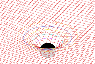
In general relativity, a geodesic generalizes the notion of a "straight line" to curved spacetime. Importantly, the world line of a particle free from all external, non-gravitational forces is a particular type of geodesic. In other words, a freely moving or falling particle always moves along a geodesic.

In physics, Maxwell's equations in curved spacetime govern the dynamics of the electromagnetic field in curved spacetime or where one uses an arbitrary coordinate system. These equations can be viewed as a generalization of the vacuum Maxwell's equations which are normally formulated in the local coordinates of flat spacetime. But because general relativity dictates that the presence of electromagnetic fields induce curvature in spacetime, Maxwell's equations in flat spacetime should be viewed as a convenient approximation.

The Newman–Penrose (NP) formalism is a set of notation developed by Ezra T. Newman and Roger Penrose for general relativity (GR). Their notation is an effort to treat general relativity in terms of spinor notation, which introduces complex forms of the usual variables used in GR. The NP formalism is itself a special case of the tetrad formalism, where the tensors of the theory are projected onto a complete vector basis at each point in spacetime. Usually this vector basis is chosen to reflect some symmetry of the spacetime, leading to simplified expressions for physical observables. In the case of the NP formalism, the vector basis chosen is a null tetrad: a set of four null vectors—two real, and a complex-conjugate pair. The two real members often asymptotically point radially inward and radially outward, and the formalism is well adapted to treatment of the propagation of radiation in curved spacetime. The Weyl scalars, derived from the Weyl tensor, are often used. In particular, it can be shown that one of these scalars— $in the appropriate frame—encodes the outgoing gravitational radiation of an asymptotically flat system.$

In probability and statistics, the quantile function outputs the value of a random variable such that its probability is less than or equal to an input probability value. Intuitively, the quantile function associates with a range at and below a probability input the likelihood that a random variable is realized in that range for some probability distribution. It is also called the percentile function, percent-point function, inverse cumulative distribution function or inverse distribution function.

In probability theory and statistics, the Conway–Maxwell–Poisson distribution is a discrete probability distribution named after Richard W. Conway, William L. Maxwell, and Siméon Denis Poisson that generalizes the Poisson distribution by adding a parameter to model overdispersion and underdispersion. It is a member of the exponential family, has the Poisson distribution and geometric distribution as special cases and the Bernoulli distribution as a limiting case.

In mathematics, the Littlewood–Richardson rule is a combinatorial description of the coefficients that arise when decomposing a product of two Schur functions as a linear combination of other Schur functions. These coefficients are natural numbers, which the Littlewood–Richardson rule describes as counting certain skew tableaux. They occur in many other mathematical contexts, for instance as multiplicity in the decomposition of tensor products of finite-dimensional representations of general linear groups, or in the decomposition of certain induced representations in the representation theory of the symmetric group, or in the area of algebraic combinatorics dealing with Young tableaux and symmetric polynomials.

In physics, quantum beats are simple examples of phenomena that cannot be described by semiclassical theory, but can be described by fully quantized calculation, especially quantum electrodynamics. In semiclassical theory (SCT), there is an interference or beat note term for both V-type and $-type atoms. However, in the quantum electrodynamic (QED) calculation, V-type atoms have a beat term but -types do not. This is strong evidence in support of quantum electrodynamics.$

In statistics, the generalized Marcum Q-function of order $is defined as$

In mathematics, Kronecker coefficientsg^λ_μν describe the decomposition of the tensor product of two irreducible representations of a symmetric group into irreducible representations. They play an important role algebraic combinatorics and geometric complexity theory. They were introduced by Murnaghan in 1938.

<span class="mw-page-title-main">Lomax distribution</span> Heavy-tail probability distribution

The Lomax distribution, conditionally also called the Pareto Type II distribution, is a heavy-tail probability distribution used in business, economics, actuarial science, queueing theory and Internet traffic modeling. It is named after K. S. Lomax. It is essentially a Pareto distribution that has been shifted so that its support begins at zero.

In the Newman–Penrose (NP) formalism of general relativity, independent components of the Ricci tensors of a four-dimensional spacetime are encoded into seven Ricci scalars which consist of three real scalars $, three complex scalars and the NP curvature scalar . Physically, Ricci-NP scalars are related with the energy-momentum distribution of the spacetime due to Einstein's field equation.$

In theoretical physics, relativistic Lagrangian mechanics is Lagrangian mechanics applied in the context of special relativity and general relativity.

In probability theory, a birth process or a pure birth process is a special case of a continuous-time Markov process and a generalisation of a Poisson process. It defines a continuous process which takes values in the natural numbers and can only increase by one or remain unchanged. This is a type of birth–death process with no deaths. The rate at which births occur is given by an exponential random variable whose parameter depends only on the current value of the process

References

↑ Marcus-Voß and Jeremie Zumer, pytwed. "Github repository". GitHub . Retrieved 2020-09-11.
↑ TraMineR. "Website on the servers of the Geneva University, CH" . Retrieved 2016-09-11.

Marteau, P.; F. (2009). "Time Warp Edit Distance with Stiffness Adjustment for Time Series Matching". IEEE Transactions on Pattern Analysis and Machine Intelligence. 31 (2): 306–318. arXiv: cs/0703033 . doi:10.1109/TPAMI.2008.76. PMID 19110495. S2CID 10049446.

This page is based on this Wikipedia article
Text is available under the CC BY-SA 4.0 license; additional terms may apply.
Images, videos and audio are available under their respective licenses.

[1] Marcus-Voß and Jeremie Zumer, pytwed. "Github repository". GitHub . Retrieved 2020-09-11.

[2] TraMineR. "Website on the servers of the Geneva University, CH" . Retrieved 2016-09-11.

[1]

[2]