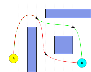
In graph theory, the shortest path problem is the problem of finding a path between two vertices in a graph such that the sum of the weights of its constituent edges is minimized.

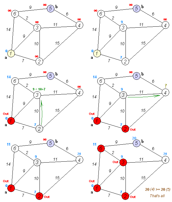
Dijkstra's algorithm is an algorithm for finding the shortest paths between nodes in a weighted graph, which may represent, for example, road networks. It was conceived by computer scientist Edsger W. Dijkstra in 1956 and published three years later.
A* is a graph traversal and pathfinding algorithm, which is used in many fields of computer science due to its completeness, optimality, and optimal efficiency. Given a weighted graph, a source node and a goal node, the algorithm finds the shortest path from source to goal.

The Bellman–Ford algorithm is an algorithm that computes shortest paths from a single source vertex to all of the other vertices in a weighted digraph. It is slower than Dijkstra's algorithm for the same problem, but more versatile, as it is capable of handling graphs in which some of the edge weights are negative numbers. The algorithm was first proposed by Alfonso Shimbel, but is instead named after Richard Bellman and Lester Ford Jr., who published it in 1958 and 1956, respectively. Edward F. Moore also published a variation of the algorithm in 1959, and for this reason it is also sometimes called the Bellman–Ford–Moore algorithm.
In computer science, the Edmonds–Karp algorithm is an implementation of the Ford–Fulkerson method for computing the maximum flow in a flow network in time. The algorithm was first published by Yefim Dinitz in 1970, and independently published by Jack Edmonds and Richard Karp in 1972. Dinitz's algorithm includes additional techniques that reduce the running time to .
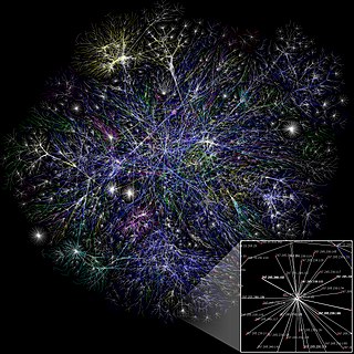
Kademlia is a distributed hash table for decentralized peer-to-peer computer networks designed by Petar Maymounkov and David Mazières in 2002. It specifies the structure of the network and the exchange of information through node lookups. Kademlia nodes communicate among themselves using UDP. A virtual or overlay network is formed by the participant nodes. Each node is identified by a number or node ID. The node ID serves not only as identification, but the Kademlia algorithm uses the node ID to locate values.
In mathematics, computer science and especially graph theory, a distance matrix is a square matrix containing the distances, taken pairwise, between the elements of a set. Depending upon the application involved, the distance being used to define this matrix may or may not be a metric. If there are N elements, this matrix will have size N×N. In graph-theoretic applications, the elements are more often referred to as points, nodes or vertices.
Route assignment, route choice, or traffic assignment concerns the selection of routes between origins and destinations in transportation networks. It is the fourth step in the conventional transportation forecasting model, following trip generation, trip distribution, and mode choice. The zonal interchange analysis of trip distribution provides origin-destination trip tables. Mode choice analysis tells which travelers will use which mode. To determine facility needs and costs and benefits, we need to know the number of travelers on each route and link of the network. We need to undertake traffic assignment. Suppose there is a network of highways and transit systems and a proposed addition. We first want to know the present pattern of traffic delay and then what would happen if the addition were made.

In graph theory and network analysis, indicators of centrality assign numbers or rankings to nodes within a graph corresponding to their network position. Applications include identifying the most influential person(s) in a social network, key infrastructure nodes in the Internet or urban networks, super-spreaders of disease, and brain networks. Centrality concepts were first developed in social network analysis, and many of the terms used to measure centrality reflect their sociological origin.

Pathfinding or pathing is the search, by a computer application, for the shortest route between two points. It is a more practical variant on solving mazes. This field of research is based heavily on Dijkstra's algorithm for finding the shortest path on a weighted graph.
Bidirectional search is a graph search algorithm that finds a shortest path from an initial vertex to a goal vertex in a directed graph. It runs two simultaneous searches: one forward from the initial state, and one backward from the goal, stopping when the two meet. The reason for this approach is that in many cases it is faster: for instance, in a simplified model of search problem complexity in which both searches expand a tree with branching factor b, and the distance from start to goal is d, each of the two searches has complexity O(bd/2) (in Big O notation), and the sum of these two search times is much less than the O(bd) complexity that would result from a single search from the beginning to the goal.
In computer science, M-trees are tree data structures that are similar to R-trees and B-trees. It is constructed using a metric and relies on the triangle inequality for efficient range and k-nearest neighbor (k-NN) queries. While M-trees can perform well in many conditions, the tree can also have large overlap and there is no clear strategy on how to best avoid overlap. In addition, it can only be used for distance functions that satisfy the triangle inequality, while many advanced dissimilarity functions used in information retrieval do not satisfy this.
In theoretical computer science and network routing, Suurballe's algorithm is an algorithm for finding two disjoint paths in a nonnegatively-weighted directed graph, so that both paths connect the same pair of vertices and have minimum total length. The algorithm was conceived by John W. Suurballe and published in 1974. The main idea of Suurballe's algorithm is to use Dijkstra's algorithm to find one path, to modify the weights of the graph edges, and then to run Dijkstra's algorithm a second time. The output of the algorithm is formed by combining these two paths, discarding edges that are traversed in opposite directions by the paths, and using the remaining edges to form the two paths to return as the output. The modification to the weights is similar to the weight modification in Johnson's algorithm, and preserves the non-negativity of the weights while allowing the second instance of Dijkstra's algorithm to find the correct second path.
In computer science, the method of contraction hierarchies is a speed-up technique for finding the shortest-path in a graph. The most intuitive applications are car-navigation systems: a user wants to drive from to using the quickest possible route. The metric optimized here is the travel time. Intersections are represented by vertices, the road sections connecting them by edges. The edge weights represent the time it takes to drive along this segment of the road. A path from to is a sequence of edges ; the shortest path is the one with the minimal sum of edge weights among all possible paths. The shortest path in a graph can be computed using Dijkstra's algorithm but, given that road networks consist of tens of millions of vertices, this is impractical. Contraction hierarchies is a speed-up method optimized to exploit properties of graphs representing road networks. The speed-up is achieved by creating shortcuts in a preprocessing phase which are then used during a shortest-path query to skip over "unimportant" vertices. This is based on the observation that road networks are highly hierarchical. Some intersections, for example highway junctions, are "more important" and higher up in the hierarchy than for example a junction leading into a dead end. Shortcuts can be used to save the precomputed distance between two important junctions such that the algorithm doesn't have to consider the full path between these junctions at query time. Contraction hierarchies do not know about which roads humans consider "important", but they are provided with the graph as input and are able to assign importance to vertices using heuristics.

The dependency network approach provides a system level analysis of the activity and topology of directed networks. The approach extracts causal topological relations between the network's nodes, and provides an important step towards inference of causal activity relations between the network nodes. This methodology has originally been introduced for the study of financial data, it has been extended and applied to other systems, such as the immune system, and semantic networks.
The k shortest path routing problem is a generalization of the shortest path routing problem in a given network. It asks not only about a shortest path but also about next k−1 shortest paths. A variation of the problem is the loopless k shortest paths.
Hierarchical closeness (HC) is a structural centrality measure used in network theory or graph theory. It is extended from closeness centrality to rank how centrally located a node is in a directed network. While the original closeness centrality of a directed network considers the most important node to be that with the least total distance from all other nodes, hierarchical closeness evaluates the most important node as the one which reaches the most nodes by the shortest paths. The hierarchical closeness explicitly includes information about the range of other nodes that can be affected by the given node. In a directed network where is the set of nodes and is the set of interactions, hierarchical closeness of a node ∈ called was proposed by Tran and Kwon as follows:
In network theory, the Wiener connector is a means of maximizing efficiency in connecting specified "query vertices" in a network. Given a connected, undirected graph and a set of query vertices in a graph, the minimum Wiener connector is an induced subgraph that connects the query vertices and minimizes the sum of shortest path distances among all pairs of vertices in the subgraph. In combinatorial optimization, the minimum Wiener connector problem is the problem of finding the minimum Wiener connector. It can be thought of as a version of the classic Steiner tree problem, where instead of minimizing the size of the tree, the objective is to minimize the distances in the subgraph.
In computer science, hub labels or the hub-labelling algorithm is a speedup technique that consumes much fewer resources than the lookup table but is still extremely fast for finding the shortest paths between nodes in a graph, which may represent, for example, road networks.
The highway dimension is a graph parameter modelling transportation networks, such as road networks or public transportation networks. It was first formally defined by Abraham et al. based on the observation by Bast et al. that any road network has a sparse set of "transit nodes", such that driving from a point A to a sufficiently far away point B along the shortest route will always pass through one of these transit nodes. It has also been proposed that the highway dimension captures the properties of public transportation networks well, given that longer routes using busses, trains, or airplanes will typically be serviced by larger transit hubs. This relates to the spoke–hub distribution paradigm in transport topology optimization.


