Transition dipole moment

Three wavefunction solutions to the time-dependent Schrödinger equation for an electron in a harmonic oscillator potential. Left: The real part (blue) and imaginary part (red) of the wavefunction. Right: The probability of finding the particle at a certain position. The top row is an energy eigenstate with low energy, the middle row is an energy eigenstate with higher energy, and the bottom is a quantum superposition mixing those two states. The bottom-right shows that the electron is moving back and forth in the superposition state. This motion causes an oscillating electric dipole moment, which in turn is proportional to the transition dipole moment between the two eigenstates.

The transition dipole moment or transition moment, usually denoted ${\displaystyle \mathbf {d} _{nm}}$ for a transition between an initial state, ${\displaystyle m}$, and a final state, ${\displaystyle n}$, is the electric dipole moment associated with the transition between the two states. In general the transition dipole moment is a complex vector quantity that includes the phase factors associated with the two states. Its direction gives the polarization of the transition, which determines how the system will interact with an electromagnetic wave of a given polarization, while the square of the magnitude gives the strength of the interaction due to the distribution of charge within the system. The SI unit of the transition dipole moment is the Coulomb-meter (Cm); a more conveniently sized unit is the Debye (D).

Definition

A single charged particle

For a transition where a single charged particle changes state from ${\displaystyle |\psi _{a}\rangle }$ to ${\displaystyle |\psi _{b}\rangle }$, the transition dipole moment ${\displaystyle {\text{(t.d.m.)}}}$ is

$${\displaystyle ({\text{t.d.m. }}a\rightarrow b)=\langle \psi _{b}|(q\mathbf {r} )|\psi _{a}\rangle =q\int \psi _{b}^{*}(\mathbf {r} )\,\mathbf {r} \,\psi _{a}(\mathbf {r} )\,d^{3}\mathbf {r} }$$

where q is the particle's charge, r is its position, and the integral is over all space (${\textstyle \int d^{3}\mathbf {r} }$ is shorthand for ${\textstyle \iiint dx\,dy\,dz}$). The transition dipole moment is a vector; for example its x-component is

$${\displaystyle ({\text{x-component of t.d.m. }}a\rightarrow b)=\langle \psi _{b}|(qx)|\psi _{a}\rangle =q\int \psi _{b}^{*}(\mathbf {r} )\,x\,\psi _{a}(\mathbf {r} )\,d^{3}\mathbf {r} }$$

In other words, the transition dipole moment can be viewed as an off-diagonal matrix element of the position operator, multiplied by the particle's charge.

Multiple charged particles

When the transition involves more than one charged particle, the transition dipole moment is defined in an analogous way to an electric dipole moment: The sum of the positions, weighted by charge. If the ith particle has charge q_i and position operator r_i, then the transition dipole moment is:

$${\displaystyle {\begin{aligned}({\text{t.d.m. }}a\rightarrow b)&=\langle \psi _{b}|(q_{1}\mathbf {r} _{1}+q_{2}\mathbf {r} _{2}+\cdots )|\psi _{a}\rangle \\&=\int \psi _{b}^{*}(\mathbf {r} _{1},\mathbf {r} _{2},\ldots )\,(q_{1}\mathbf {r} _{1}+q_{2}\mathbf {r} _{2}+\cdots )\,\psi _{a}(\mathbf {r} _{1},\mathbf {r} _{2},\ldots )\,d^{3}\mathbf {r} _{1}\,d^{3}\mathbf {r} _{2}\cdots \end{aligned}}}$$

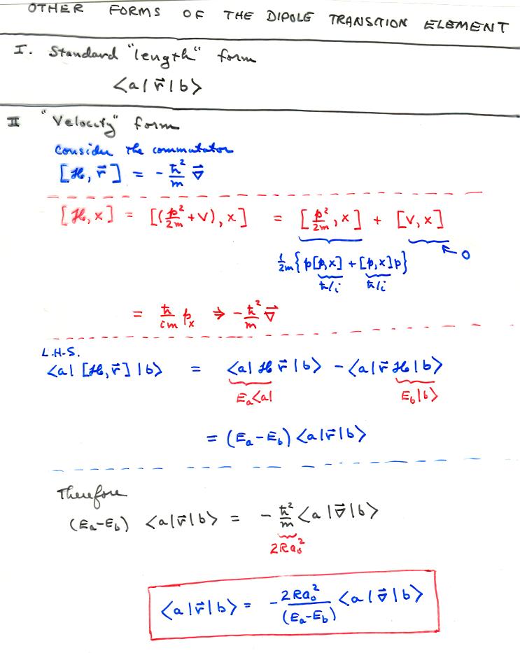
In terms of momentum

For a single, nonrelativistic particle of mass m, in zero magnetic field, the transition dipole moment between two energy eigenstates ψ_a and ψ_b can alternatively be written in terms of the momentum operator, using the relationship ^[1]

$${\displaystyle \langle \psi _{a}|\mathbf {r} |\psi _{b}\rangle ={\frac {i\hbar }{(E_{b}-E_{a})m}}\langle \psi _{a}|\mathbf {p} |\psi _{b}\rangle }$$

This relationship can be proven starting from the commutation relation between position x and the Hamiltonian H:

$${\displaystyle [H,x]=\left[{\frac {p^{2}}{2m}}+V(x,y,z),x\right]=\left[{\frac {p^{2}}{2m}},x\right]={\frac {1}{2m}}(p_{x}[p_{x},x]+[p_{x},x]p_{x})={\frac {-i\hbar p_{x}}{m}}}$$

Then

$${\displaystyle \langle \psi _{a}|(Hx-xH)|\psi _{b}\rangle ={\frac {-i\hbar }{m}}\langle \psi _{a}|p_{x}|\psi _{b}\rangle }$$

However, assuming that ψ_a and ψ_b are energy eigenstates with energy E_a and E_b, we can also write

$${\displaystyle \langle \psi _{a}|(Hx-xH)|\psi _{b}\rangle =(\langle \psi _{a}|H)x|\psi _{b}\rangle -\langle \psi _{a}|x(H|\psi _{b}\rangle )=(E_{a}-E_{b})\langle \psi _{a}|x|\psi _{b}\rangle }$$

Similar relations hold for y and z, which together give the relationship above.

Analogy with a classical dipole

Main article: Electric dipole moment

A basic, phenomenological understanding of the transition dipole moment can be obtained by analogy with a classical dipole. While the comparison can be very useful, care must be taken to ensure that one does not fall into the trap of assuming they are the same.

In the case of two classical point charges, ${\displaystyle +q}$ and ${\displaystyle -q}$, with a displacement vector, ${\displaystyle \mathbf {r} }$, pointing from the negative charge to the positive charge, the electric dipole moment is given by

$${\displaystyle \mathbf {p} =q\mathbf {r} .}$$

In the presence of an electric field, such as that due to an electromagnetic wave, the two charges will experience a force in opposite directions, leading to a net torque on the dipole. The magnitude of the torque is proportional to both the magnitude of the charges and the separation between them, and varies with the relative angles of the field and the dipole:

$${\displaystyle \left|\mathbf {\tau } \right|=\left|q\mathbf {r} \right|\left|\mathbf {E} \right|\sin \theta .}$$

Similarly, the coupling between an electromagnetic wave and an atomic transition with transition dipole moment ${\displaystyle \mathbf {d} _{nm}}$ depends on the charge distribution within the atom, the strength of the electric field, and the relative polarizations of the field and the transition. In addition, the transition dipole moment depends on the geometries and relative phases of the initial and final states.

Origin

When an atom or molecule interacts with an electromagnetic wave of frequency ${\displaystyle \omega }$, it can undergo a transition from an initial to a final state of energy difference ${\displaystyle \hbar \omega }$ through the coupling of the electromagnetic field to the transition dipole moment. When this transition is from a lower energy state to a higher energy state, this results in the absorption of a photon. A transition from a higher energy state to a lower energy state results in the emission of a photon. If the charge, ${\displaystyle e}$, is omitted from the electric dipole operator during this calculation, one obtains ${\displaystyle \mathbf {R} _{\alpha }}$ as used in oscillator strength.

Applications

The transition dipole moment is useful for determining if transitions are allowed under the electric dipole interaction. For example, the transition from a bonding ${\displaystyle \pi }$ orbital to an antibonding ${\displaystyle \pi ^{*}}$ orbital is allowed because the integral defining the transition dipole moment is nonzero. Such a transition occurs between an even and an odd orbital; the dipole operator, ${\displaystyle {\vec {\mu }}}$, is an odd function of ${\displaystyle \mathbf {r} }$, hence the integrand is an even function. The integral of an odd function over symmetric limits returns a value of zero, while for an even function this is not necessarily the case. This result is reflected in the parity selection rule for electric dipole transitions. The transition moment integral

$${\displaystyle \int \psi _{1}^{*}{\vec {\mu }}\psi _{2}d\tau ,}$$

of an electronic transition within similar atomic orbitals, such as s-s or p-p, is forbidden due to the triple integral returning an ungerade (odd) product. Such transitions only redistribute electrons within the same orbital and will return a zero product. If the triple integral returns a gerade (even) product, the transition is allowed.

See also

• Wigner–Eckart theorem

References

1. lecture notes on electric dipole radiation, especially length vs velocity

"IUPAC compendium of Chemical Terminology". IUPAC. 1997. doi:10.1351/goldbook.T06460 . Retrieved 2007-01-15.