The method of least squares is a standard approach in regression analysis to approximate the solution of overdetermined systems by minimizing the sum of the squares of the residuals made in the results of each individual equation.

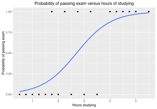
In statistics, the logistic model is a statistical model that models the probability of an event taking place by having the log-odds for the event be a linear combination of one or more independent variables. In regression analysis, logistic regression is estimating the parameters of a logistic model. Formally, in binary logistic regression there is a single binary dependent variable, coded by an indicator variable, where the two values are labeled "0" and "1", while the independent variables can each be a binary variable or a continuous variable. The corresponding probability of the value labeled "1" can vary between 0 and 1, hence the labeling; the function that converts log-odds to probability is the logistic function, hence the name. The unit of measurement for the log-odds scale is called a logit, from logistic unit, hence the alternative names. See § Background and § Definition for formal mathematics, and § Example for a worked example.
Survival analysis is a branch of statistics for analyzing the expected duration of time until one event occurs, such as death in biological organisms and failure in mechanical systems. This topic is called reliability theory or reliability analysis in engineering, duration analysis or duration modelling in economics, and event history analysis in sociology. Survival analysis attempts to answer certain questions, such as what is the proportion of a population which will survive past a certain time? Of those that survive, at what rate will they die or fail? Can multiple causes of death or failure be taken into account? How do particular circumstances or characteristics increase or decrease the probability of survival?
The Akaike information criterion (AIC) is an estimator of prediction error and thereby relative quality of statistical models for a given set of data. Given a collection of models for the data, AIC estimates the quality of each model, relative to each of the other models. Thus, AIC provides a means for model selection.

In statistical modeling, regression analysis is a set of statistical processes for estimating the relationships between a dependent variable and one or more independent variables. The most common form of regression analysis is linear regression, in which one finds the line that most closely fits the data according to a specific mathematical criterion. For example, the method of ordinary least squares computes the unique line that minimizes the sum of squared differences between the true data and that line. For specific mathematical reasons, this allows the researcher to estimate the conditional expectation of the dependent variable when the independent variables take on a given set of values. Less common forms of regression use slightly different procedures to estimate alternative location parameters or estimate the conditional expectation across a broader collection of non-linear models.
In statistics, a probit model is a type of regression where the dependent variable can take only two values, for example married or not married. The word is a portmanteau, coming from probability + unit. The purpose of the model is to estimate the probability that an observation with particular characteristics will fall into a specific one of the categories; moreover, classifying observations based on their predicted probabilities is a type of binary classification model.
In statistics, ordinary least squares (OLS) is a type of linear least squares method for choosing the unknown parameters in a linear regression model by the principle of least squares: minimizing the sum of the squares of the differences between the observed dependent variable in the input dataset and the output of the (linear) function of the independent variable.
This glossary of statistics and probability is a list of definitions of terms and concepts used in the mathematical sciences of statistics and probability, their sub-disciplines, and related fields. For additional related terms, see Glossary of mathematics and Glossary of experimental design.
In statistics, a tobit model is any of a class of regression models in which the observed range of the dependent variable is censored in some way. The term was coined by Arthur Goldberger in reference to James Tobin, who developed the model in 1958 to mitigate the problem of zero-inflated data for observations of household expenditure on durable goods. Because Tobin's method can be easily extended to handle truncated and other non-randomly selected samples, some authors adopt a broader definition of the tobit model that includes these cases.
Truncated regression models are a class of models in which the sample has been truncated for certain ranges of the dependent variable. That means observations with values in the dependent variable below or above certain thresholds are systematically excluded from the sample. Therefore, whole observations are missing, so that neither the dependent nor the independent variable is known. This is in contrast to censored regression models where only the value of the dependent variable is clustered at a lower threshold, an upper threshold, or both, while the value for independent variables is available.
Bootstrapping is any test or metric that uses random sampling with replacement, and falls under the broader class of resampling methods. Bootstrapping assigns measures of accuracy to sample estimates. This technique allows estimation of the sampling distribution of almost any statistic using random sampling methods.
Omnibus tests are a kind of statistical test. They test whether the explained variance in a set of data is significantly greater than the unexplained variance, overall. One example is the F-test in the analysis of variance. There can be legitimate significant effects within a model even if the omnibus test is not significant. For instance, in a model with two independent variables, if only one variable exerts a significant effect on the dependent variable and the other does not, then the omnibus test may be non-significant. This fact does not affect the conclusions that may be drawn from the one significant variable. In order to test effects within an omnibus test, researchers often use contrasts.
In statistics, censoring is a condition in which the value of a measurement or observation is only partially known.

Quantile regression is a type of regression analysis used in statistics and econometrics. Whereas the method of least squares estimates the conditional mean of the response variable across values of the predictor variables, quantile regression estimates the conditional median of the response variable. Quantile regression is an extension of linear regression used when the conditions of linear regression are not met.
The Heckman correction is a statistical technique to correct bias from non-randomly selected samples or otherwise incidentally truncated dependent variables, a pervasive issue in quantitative social sciences when using observational data. Conceptually, this is achieved by explicitly modelling the individual sampling probability of each observation together with the conditional expectation of the dependent variable. The resulting likelihood function is mathematically similar to the tobit model for censored dependent variables, a connection first drawn by James Heckman in 1974. Heckman also developed a two-step control function approach to estimate this model, which avoids the computational burden of having to estimate both equations jointly, albeit at the cost of inefficiency. Heckman received the Nobel Memorial Prize in Economic Sciences in 2000 for his work in this field.
In probability theory, the Mills ratio of a continuous random variable is the function
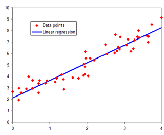
In statistics, linear regression is a linear approach for modelling the relationship between a scalar response and one or more explanatory variables. The case of one explanatory variable is called simple linear regression; for more than one, the process is called multiple linear regression. This term is distinct from multivariate linear regression, where multiple correlated dependent variables are predicted, rather than a single scalar variable.
In statistics, the class of vector generalized linear models (VGLMs) was proposed to enlarge the scope of models catered for by generalized linear models (GLMs). In particular, VGLMs allow for response variables outside the classical exponential family and for more than one parameter. Each parameter can be transformed by a link function. The VGLM framework is also large enough to naturally accommodate multiple responses; these are several independent responses each coming from a particular statistical distribution with possibly different parameter values.

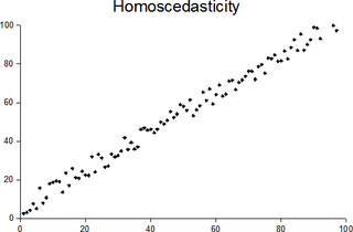
In statistics, a sequence of random variables is homoscedastic if all its random variables have the same finite variance; this is also known as homogeneity of variance. The complementary notion is called heteroscedasticity, also known as heterogeneity of variance. The spellings homoskedasticity and heteroskedasticity are also frequently used. Assuming a variable is homoscedastic when in reality it is heteroscedastic results in unbiased but inefficient point estimates and in biased estimates of standard errors, and may result in overestimating the goodness of fit as measured by the Pearson coefficient.


