Envelope (mathematics)

For the envelope of an oscillating signal, see Envelope (waves). For the abstract concept, see Envelope (category theory).

Construction of the envelope of a family of curves.

In geometry, an envelope of a planar family of curves is a curve that is tangent to each member of the family at some point, and these points of tangency together form the whole envelope. Classically, a point on the envelope can be thought of as the intersection of two "infinitesimally adjacent" curves, meaning the limit of intersections of nearby curves. This idea can be generalized to an envelope of surfaces in space, and so on to higher dimensions.

To have an envelope, it is necessary that the individual members of the family of curves are differentiable curves as the concept of tangency does not apply otherwise, and there has to be a smooth transition proceeding through the members. But these conditions are not sufficient – a given family may fail to have an envelope. A simple example of this is given by a family of concentric circles of expanding radius.

Envelope of a family of curves

Let each curve ${\displaystyle C_{t}}$ in the family be given as the solution of an equation ${\displaystyle f_{t}(x,y)=0}$ (see implicit curve), where ${\displaystyle t}$ is a parameter. Write ${\displaystyle F(t,x,y)=f_{t}(x,y)}$ and assume ${\displaystyle F}$ is differentiable.

The envelope of the family ${\displaystyle C_{t}}$ is then defined as the set ${\displaystyle {\mathcal {D}}}$ of points ${\displaystyle (x,y)}$ for which, simultaneously,

${\displaystyle F(t,x,y)=0~~{\mathsf {and}}~~{\partial F \over \partial t}(t,x,y)=0}$

for some value of ${\displaystyle t}$, where ${\displaystyle \partial F/\partial t}$ is the partial derivative of ${\displaystyle F}$ with respect to ${\displaystyle t}$. ^[1]

If ${\displaystyle t}$ and ${\displaystyle u}$, ${\displaystyle t\neq u}$ are two values of the parameter then the intersection of the curves ${\displaystyle C_{t}}$ and ${\displaystyle C_{u}}$ is given by

${\displaystyle F(t,x,y)=F(u,x,y)=0\,}$

or, equivalently,

${\displaystyle F(t,x,y)=0~~{\mathsf {and}}~~{\frac {F(u,x,y)-F(t,x,y)}{u-t}}=0.}$

Letting ${\displaystyle u\to t}$ gives the definition above.

An important special case is when ${\displaystyle F(t,x,y)}$ is a polynomial in ${\displaystyle t}$. This includes, by clearing denominators, the case where ${\displaystyle F(t,x,y)}$ is a rational function in ${\displaystyle t}$. In this case, the definition amounts to ${\displaystyle t}$ being a double root of ${\displaystyle F(t,x,y)}$, so the equation of the envelope can be found by setting the discriminant of ${\displaystyle F}$ to ${\displaystyle 0}$ (because the definition demands ${\displaystyle F=0}$ at some ${\displaystyle t}$ and first derivative ${\displaystyle F=0}$ i.e. its value ${\displaystyle 0}$ and it is min/max at that ${\displaystyle t}$).

For example, let ${\displaystyle C_{t}}$ be the line whose ${\displaystyle x}$ and ${\displaystyle y}$ intercepts are ${\displaystyle t}$ and ${\displaystyle 11-t}$, this is shown in the animation above. The equation of ${\displaystyle C_{t}}$ is

${\displaystyle {\frac {x}{t}}+{\frac {y}{11-t}}=1}$

or, clearing fractions,

${\displaystyle x(11-t)+yt-t(11-t)=t^{2}+(-x+y-11)t+11x=0.\,}$

The equation of the envelope is then

${\displaystyle (-x+y-11)^{2}-44x=(x-y)^{2}-22(x+y)+121=0.\,}$

Often when ${\displaystyle F}$ is not a rational function of the parameter it may be reduced to this case by an appropriate substitution. For example, if the family is given by ${\displaystyle C_{\theta }}$ with an equation of the form ${\displaystyle u(x,y)\cos \theta +v(x,y)\sin \theta =w(x,y)}$, then putting ${\displaystyle t=e^{i\theta }}$ , ${\displaystyle \cos \theta =(t+1/t)/2}$, ${\displaystyle \sin \theta =(t-1/t)/2i}$ changes the equation of the curve to

${\displaystyle u{1 \over 2}\left(t+{1 \over t}\right)+v{1 \over 2i}\left(t-{1 \over t}\right)=w}$

or

${\displaystyle (u-iv)t^{2}-2wt+(u+iv)=0.\,}$

The equation of the envelope is then given by setting the discriminant to ${\displaystyle 0}$:

${\displaystyle (u-iv)(u+iv)-w^{2}=0\,}$

or

${\displaystyle u^{2}+v^{2}=w^{2}.\,}$

Alternative definitions

1. The envelope ${\displaystyle E_{1}}$ is the limit of intersections of nearby curves ${\displaystyle C_{t}}$.
2. The envelope ${\displaystyle E_{2}}$ is a curve tangent to all of the ${\displaystyle C_{t}}$.
3. The envelope ${\displaystyle E_{3}}$ is the boundary of the region filled by the curves ${\displaystyle C_{t}}$.

Then ${\displaystyle E_{1}\subseteq {\mathcal {D}}}$, ${\displaystyle E_{2}\subseteq {\mathcal {D}}}$ and ${\displaystyle E_{3}\subseteq {\mathcal {D}}}$, where ${\displaystyle {\mathcal {D}}}$ is the set of points defined at the beginning of this subsection's parent section.

Examples

Example 1

These definitions ${\displaystyle E_{1}}$, ${\displaystyle E_{2}}$, and ${\displaystyle E_{3}}$ of the envelope may be different sets. Consider for instance the curve ${\displaystyle y=x^{3}}$ parametrised by ${\displaystyle \gamma$ :\mathbb {R} \to \mathbb {R} ^{2}} where ${\displaystyle \gamma (t)=(t,t^{3})}$. The one-parameter family of curves will be given by the tangent lines to ${\displaystyle \gamma }$.

First we calculate the discriminant ${\displaystyle {\mathcal {D}}}$. The generating function is

${\displaystyle F(t,(x,y))=3t^{2}x-y-2t^{3}.}$

Calculating the partial derivative ${\displaystyle F_{t}=6t(x-t)}$. It follows that either ${\displaystyle x=t}$ or ${\displaystyle t=0}$. First assume that ${\displaystyle x=t}$ and ${\displaystyle t\neq 0}$. Substituting into ${\displaystyle F}$: ${\displaystyle F(t,(t,y))=t^{3}-y\,}$ and so, assuming that ${\displaystyle t\neq 0}$, it follows that ${\displaystyle F=F_{t}=0}$ if and only if ${\displaystyle (x,y)=(t,t^{3})}$. Next, assuming that ${\displaystyle t=0}$ and substituting into ${\displaystyle F}$ gives ${\displaystyle F(0,(x,y))=-y}$. So, assuming ${\displaystyle t=0}$, it follows that ${\displaystyle F=F_{t}=0}$ if and only if ${\displaystyle y=0}$. Thus the discriminant is the original curve and its tangent line at ${\displaystyle \gamma (0)}$:

${\displaystyle {\mathcal {D}}=\{(x,y)\in \mathbb {R} ^{2}:y=x^{3}\}\cup \{(x,y)\in \mathbb {R} ^{2}:y=0\}\ .}$

Next we calculate ${\displaystyle E_{1}}$. One curve is given by ${\displaystyle F(t,(x,y))=0}$ and a nearby curve is given by ${\displaystyle F(t+\varepsilon ,(x,y))=0}$ where ${\displaystyle \varepsilon }$ is some very small number. The intersection point comes from looking at the limit of ${\displaystyle F(t,(x,y))=F(t+\varepsilon ,(x,y))}$ as ${\displaystyle \varepsilon }$ tends to zero. Notice that ${\displaystyle F(t,(x,y))=F(t+\varepsilon ,(x,y))}$ if and only if

${\displaystyle L:=F(t,(x,y))-F(t+\varepsilon ,(x,y))=2\varepsilon ^{3}+6\varepsilon t^{2}+6\varepsilon ^{2}t-(3\varepsilon ^{2}+6\varepsilon t)x=0.}$

If ${\displaystyle t\neq 0}$ then ${\displaystyle L}$ has only a single factor of ${\displaystyle \varepsilon }$. Assuming that ${\displaystyle t\neq 0}$ then the intersection is given by

${\displaystyle \lim _{\varepsilon \to 0}{\frac {1}{\varepsilon }}L=6t(t-x)\ .}$

Since ${\displaystyle t\neq 0}$ it follows that ${\displaystyle x=t}$. The ${\displaystyle y}$ value is calculated by knowing that this point must lie on a tangent line to the original curve ${\displaystyle \gamma }$: that ${\displaystyle F(t,(x,y))=0}$. Substituting and solving gives ${\displaystyle y=t^{3}}$. When ${\displaystyle t=0}$, ${\displaystyle L}$ is divisible by ${\displaystyle \varepsilon ^{2}}$. Assuming that ${\displaystyle t=0}$ then the intersection is given by

${\displaystyle \lim _{\varepsilon \to 0}{\frac {1}{\varepsilon ^{2}}}L=3x\ .}$

It follows that ${\displaystyle x=0}$, and knowing that ${\displaystyle F(t,(x,y))=0}$ gives ${\displaystyle y=0}$. It follows that

${\displaystyle E_{1}=\{(x,y)\in \mathbb {R} ^{2}:y=x^{3}\}\ .}$

Next we calculate ${\displaystyle E_{2}}$. The curve itself is the curve that is tangent to all of its own tangent lines. It follows that

${\displaystyle E_{2}=\{(x,y)\in \mathbb {R} ^{2}:y=x^{3}\}\ .}$

Finally we calculate ${\displaystyle E_{3}}$. Every point in the plane has at least one tangent line to ${\displaystyle \gamma }$ passing through it, and so region filled by the tangent lines is the whole plane. The boundary ${\displaystyle E_{3}}$ is therefore the empty set. Indeed, consider a point in the plane, say ${\displaystyle (x_{0},y_{0})}$. This point lies on a tangent line if and only if there exists a ${\displaystyle t}$ such that

${\displaystyle F(t,(x_{0},y_{0}))=3t^{2}x_{0}-y_{0}-2t^{3}=0\ .}$

This is a cubic in ${\displaystyle t}$ and as such has at least one real solution. It follows that at least one tangent line to ${\displaystyle \gamma }$ must pass through any given point in the plane. If ${\displaystyle y>x^{3}}$ and ${\displaystyle y>0}$ then each point ${\displaystyle (x,y)}$ has exactly one tangent line to ${\displaystyle \gamma }$ passing through it. The same is true if ${\displaystyle y<x^{3}}$ and ${\displaystyle y<0}$. If ${\displaystyle y<x^{3}}$ and ${\displaystyle y>0}$ then each point ${\displaystyle (x,y)}$ has exactly three distinct tangent lines to ${\displaystyle \gamma }$ passing through it. The same is true if ${\displaystyle y>x^{3}}$ and ${\displaystyle y<0}$. If ${\displaystyle y=x^{3}}$ and ${\displaystyle y\neq 0}$ then each point ${\displaystyle (x,y)}$ has exactly two tangent lines to ${\displaystyle \gamma }$ passing through it (this corresponds to the cubic having one ordinary root and one repeated root). The same is true if ${\displaystyle y\neq x^{3}}$ and ${\displaystyle y=0}$. If ${\displaystyle y=x^{3}}$ and ${\displaystyle x=0}$, i.e., ${\displaystyle x=y=0}$, then this point has a single tangent line to ${\displaystyle \gamma }$ passing through it (this corresponds to the cubic having one real root of multiplicity 3). It follows that

${\displaystyle E_{3}=\varnothing .}$

Example 2

This plot gives the envelope of the family of lines connecting points (t,0), (0,k - t), in which k takes the value 1.

In string art it is common to cross-connect two lines of equally spaced pins. What curve is formed?

For simplicity, set the pins on the ${\displaystyle x}$- and ${\displaystyle y}$-axes; a non-orthogonal layout is a rotation and scaling away. A general straight-line thread connects the two points ${\displaystyle (0,k-t)}$ and ${\displaystyle (t,0)}$, where ${\displaystyle k}$ is an arbitrary scaling constant, and the family of lines is generated by varying the parameter ${\displaystyle t}$. From simple geometry, the equation of this straight line is ${\displaystyle y=-(k-t)x/t+k-t}$. Rearranging and casting in the form ${\displaystyle F(x,y,t)=0}$ gives:

${\displaystyle F(x,y,t)=-{\frac {kx}{t}}-t+x+k-y=0\,}$

1

Now differentiate ${\displaystyle F(x,y,t)}$ with respect to ${\displaystyle t}$ and set the result equal to zero, to get

${\displaystyle {\frac {\partial F(x,y,t)}{\partial t}}={\frac {kx}{t^{2}}}-1=0\,}$

2

These two equations jointly define the equation of the envelope. From (2) we have:

${\displaystyle t={\sqrt {kx}}\,}$

Substituting this value of ${\displaystyle t}$ into (1) and simplifying gives an equation for the envelope:

${\displaystyle y=({\sqrt {x}}-{\sqrt {k}})^{2}\,}$

3

Or, rearranging into a more elegant form that shows the symmetry between ${\displaystyle x}$ and ${\displaystyle y}$:

${\displaystyle {\sqrt {x}}+{\sqrt {y}}={\sqrt {k}}}$

4

We can take a rotation of the axes where the ${\displaystyle b}$ axis is the line ${\displaystyle y=x}$ oriented northeast and the ${\displaystyle a}$ axis is the line ${\displaystyle y=-x}$ oriented southeast. These new axes are related to the original ${\displaystyle x-y}$ axes by ${\displaystyle x=(b+a)/{\sqrt {2}}}$ and ${\displaystyle y=(b-a)/{\sqrt {2}}}$ . We obtain, after substitution into (4) and expansion and simplification,

${\displaystyle b={\frac {1}{k{\sqrt {2}}}}a^{2}+{\frac {k}{2{\sqrt {2}}}},}$

5

which is apparently the equation for a parabola with axis along ${\displaystyle a=0}$, or ${\displaystyle y=x}$.

Example 3

Let ${\displaystyle I\subset \mathbb {R} }$ be an open interval and let ${\displaystyle \gamma :I\to \mathbb {R} ^{2}}$ be a smooth plane curve parametrised by arc length. Consider the one-parameter family of normal lines to ${\displaystyle \gamma (I)}$. A line is normal to ${\displaystyle \gamma }$ at ${\displaystyle \gamma (t)}$ if it passes through ${\displaystyle \gamma (t)}$ and is perpendicular to the tangent vector to ${\displaystyle \gamma }$ at ${\displaystyle \gamma (t)}$. Let ${\displaystyle \mathbf {T} }$ denote the unit tangent vector to ${\displaystyle \gamma }$ and let ${\displaystyle \mathbf {N} }$ denote the unit normal vector. Using a dot to denote the dot product, the generating family for the one-parameter family of normal lines is given by ${\displaystyle F:I\times \mathbb {R} ^{2}\to \mathbb {R} }$ where

${\displaystyle F(t,{\mathbf {x} })=({\mathbf {x} }-\gamma (t))\cdot {\mathbf {T} }(t)\ .}$

Clearly ${\displaystyle (x-y)\cdot \mathbf {T} =0}$ if and only if ${\displaystyle x-\gamma }$ is perpendicular to ${\displaystyle \mathbf {T} }$, or equivalently, if and only if ${\displaystyle x-\gamma }$ is parallel to ${\displaystyle \mathbf {N} }$, or equivalently, if and only if ${\displaystyle x=\gamma +\lambda \mathbf {N} }$ for some λ ∈ R. It follows that

${\displaystyle L_{t_{0}}:=\{{\mathbf {x} }\in \mathbb {R} ^{2}:F(t_{0},{\mathbf {x} })=0\}}$

is exactly the normal line to ${\displaystyle \gamma }$ at ${\displaystyle \gamma (t_{0})}$. To find the discriminant of ${\displaystyle F}$ we need to compute its partial derivative with respect to ${\displaystyle t}$:

${\displaystyle {\frac {\partial F}{\partial t}}(t,{\mathbf {x} })=\kappa (t)({\mathbf {x} }-\gamma (t))\cdot {\mathbf {N} }(t)-1\ ,}$

where ${\displaystyle \kappa }$ is the plane curve curvature of ${\displaystyle \gamma }$. It has been seen that ${\displaystyle F=0}$ if and only if ${\displaystyle x-\gamma =\lambda \mathbf {N} }$ for some ${\displaystyle \lambda \in \mathbb {R} }$. Assuming that ${\displaystyle F=0}$ gives

${\displaystyle {\frac {\partial F}{\partial t}}=\lambda \kappa (t)-1\ .}$

Assuming that ${\displaystyle \kappa \neq 0}$ it follows that ${\displaystyle \lambda =1/\kappa }$ and so

${\displaystyle {\mathcal {D}}=\gamma (t)+{\frac {1}{\kappa (t)}}{\mathbf {N} }(t)\ .}$

This is exactly the evolute of the curve ${\displaystyle \gamma }$.

Example 4

An astroid as the envelope of the family of lines connecting points (s,0), (0,t) with s + t = 1

The following example shows that in some cases the envelope of a family of curves may be seen as the topologic boundary of a union of sets, whose boundaries are the curves of the envelope. For ${\displaystyle s>0}$ and ${\displaystyle t>0}$ consider the (open) right triangle in a Cartesian plane with vertices ${\displaystyle (0,0)}$, ${\displaystyle (s,0)}$ and ${\displaystyle (0,t)}$

${\displaystyle T_{s,t}:=\left\{(x,y)\in \mathbb {R} _{+}^{2}:\ {\frac {x}{s}}+{\frac {y}{t}}<1\right\}.}$

Fix an exponent ${\displaystyle \alpha >0}$, and consider the union of all the triangles ${\displaystyle T_{s,t}}$ subjected to the constraint ${\displaystyle \textstyle s^{\alpha }+t^{\alpha }=1}$, that is the open set

${\displaystyle \Delta _{\alpha }:=\bigcup _{s^{\alpha }+t^{\alpha }=1}T_{s,t}.}$

To write a Cartesian representation for ${\displaystyle \textstyle \Delta _{\alpha }}$, start with any ${\displaystyle \textstyle s>0}$, ${\displaystyle \textstyle t>0}$ satisfying ${\displaystyle \textstyle s^{\alpha }+t^{\alpha }=1}$ and any ${\displaystyle \textstyle (x,y)\in \mathbb {R} _{+}^{2}}$. The Hölder inequality in ${\displaystyle \textstyle \mathbb {R} ^{2}}$ with respect to the conjugated exponents ${\displaystyle p:=1+{\frac {1}{\alpha }}}$ and ${\displaystyle \textstyle q:={1+\alpha }}$ gives:

${\displaystyle x^{\frac {\alpha }{\alpha +1}}+y^{\frac {\alpha }{\alpha +1}}\leq \left({\frac {x}{s}}+{\frac {y}{t}}\right)^{\frac {\alpha }{\alpha +1}}{\Big (}s^{\alpha }+t^{\alpha }{\Big )}^{\frac {1}{\alpha +1}}=\left({\frac {x}{s}}+{\frac {y}{t}}\right)^{\frac {\alpha }{\alpha +1}}}$,

with equality if and only if ${\displaystyle \textstyle s:\,t=x^{\frac {1}{1+\alpha }}:\,y^{\frac {1}{1+\alpha }}}$. In terms of a union of sets the latter inequality reads: the point ${\displaystyle (x,y)\in \mathbb {R} _{+}^{2}}$ belongs to the set ${\displaystyle \textstyle \Delta _{\alpha }}$, that is, it belongs to some ${\displaystyle \textstyle T_{s,t}}$ with ${\displaystyle \textstyle s^{\alpha }+t^{\alpha }=1}$, if and only if it satisfies

${\displaystyle x^{\frac {\alpha }{\alpha +1}}+y^{\frac {\alpha }{\alpha +1}}<1.}$

Moreover, the boundary in ${\displaystyle \mathbb {R} _{+}^{2}}$ of the set ${\displaystyle \textstyle \Delta _{\alpha }}$ is the envelope of the corresponding family of line segments

${\displaystyle \left\{(x,y)\in \mathbb {R} _{+}^{2}:\ {\frac {x}{s}}+{\frac {y}{t}}=1\right\}\ ,\qquad s^{\alpha }+t^{\alpha }=1}$

(that is, the hypotenuses of the triangles), and has Cartesian equation

${\displaystyle x^{\frac {\alpha }{\alpha +1}}+y^{\frac {\alpha }{\alpha +1}}=1.}$

Notice that, in particular, the value ${\displaystyle \alpha =1}$ gives the arc of parabola of the Example 2, and the value ${\displaystyle \alpha =2}$ (meaning that all hypotenuses are unit length segments) gives the astroid.

Example 5

The orbits' envelope of the projectiles (with constant initial speed) is a concave parabola. The initial speed is 10 m/s. We take g = 10 m/s .

We consider the following example of envelope in motion. Suppose at initial height ${\displaystyle 0}$, one casts a projectile into the air with constant initial velocity ${\displaystyle v}$ but different elevation angles ${\displaystyle \theta }$. Let ${\displaystyle x}$ be the horizontal axis in the motion surface, and let ${\displaystyle y}$ denote the vertical axis. Then the motion gives the following differential dynamical system:

${\displaystyle {\frac {d^{2}y}{dt^{2}}}=-g,\;{\frac {d^{2}x}{dt^{2}}}=0,}$

which satisfies four initial conditions:

${\displaystyle {\frac {dx}{dt}}{\bigg |}_{t=0}=v\cos \theta ,\;{\frac {dy}{dt}}{\bigg |}_{t=0}=v\sin \theta ,\;x{\bigg |}_{t=0}=y{\bigg |}_{t=0}=0.}$

Here ${\displaystyle t}$ denotes motion time, ${\displaystyle \theta }$ is elevation angle, ${\displaystyle g}$ denotes gravitational acceleration, and ${\displaystyle v}$ is the constant initial speed (not velocity). The solution of the above system can take an implicit form:

${\displaystyle F(x,y,\theta )=x\tan \theta -{\frac {gx^{2}}{2v^{2}\cos ^{2}\theta }}-y=0.}$

To find its envelope equation, one may compute the desired derivative:

${\displaystyle {\frac {\partial F}{\partial \theta }}={\frac {x}{\cos ^{2}\theta }}-{\frac {gx^{2}\tan \theta }{v^{2}\cos ^{2}\theta }}=0.}$

By eliminating ${\displaystyle \theta }$, one may reach the following envelope equation:

${\displaystyle y={\frac {v^{2}}{2g}}-{\frac {g}{2v^{2}}}x^{2}.}$

Clearly the resulted envelope is also a concave parabola.

Envelope of a family of surfaces

A one-parameter family of surfaces in three-dimensional Euclidean space is given by a set of equations

${\displaystyle F(x,y,z,a)=0}$

depending on a real parameter ${\displaystyle a}$. ^[2] For example, the tangent planes to a surface along a curve in the surface form such a family.

Two surfaces corresponding to different values ${\displaystyle a}$ and ${\displaystyle a'}$ intersect in a common curve defined by

${\displaystyle F(x,y,z,a)=0,\,\,{F(x,y,z,a^{\prime })-F(x,y,z,a) \over a^{\prime }-a}=0.}$

In the limit as ${\displaystyle a'}$ approaches ${\displaystyle a}$, this curve tends to a curve contained in the surface at ${\displaystyle a}$

${\displaystyle F(x,y,z,a)=0,\,\,{\partial F \over \partial a}(x,y,z,a)=0.}$

This curve is called the characteristic of the family at ${\displaystyle a}$. As ${\displaystyle a}$ varies the locus of these characteristic curves defines a surface called the envelope of the family of surfaces.

The envelope of a family of surfaces is tangent to each surface in the family along the characteristic curve in that surface.

Generalisations

The idea of an envelope of a family of smooth submanifolds follows naturally. In general, if we have a family of submanifolds with codimension ${\displaystyle c}$ then we need to have at least a ${\displaystyle c}$-parameter family of such submanifolds. For example: a one-parameter family of curves in three-space (${\displaystyle c=2}$) does not, generically, have an envelope.

Applications

Ordinary differential equations

Envelopes are connected to the study of ordinary differential equations (ODEs), and in particular singular solutions of ODEs. ^[3] Consider, for example, the one-parameter family of tangent lines to the parabola ${\displaystyle y=x^{2}}$. These are given by the generating family ${\displaystyle F(t,(x,y))=t^{2}-2tx+y}$. The zero level set ${\displaystyle F(t_{0},(x,y))=0}$ gives the equation of the tangent line to the parabola at the point ${\displaystyle (t_{0},t_{0}^{2})}$. The equation ${\displaystyle t^{2}-2tx+y=0}$ can always be solved for ${\displaystyle y}$ as a function of ${\displaystyle x}$ and so, consider

${\displaystyle t^{2}-2tx+y(x)=0.\ }$

Substituting

${\displaystyle t=\left({\frac {dy}{dx}}\right)/2}$

gives the ODE

${\displaystyle \left({\frac {dy}{dx}}\right)^{2}\!\!-4x{\frac {dy}{dx}}+4y=0.}$

Not surprisingly ${\displaystyle y=2tx-t^{2}}$ are all solutions to this ODE. However, the envelope of this one-parameter family of lines, which is the parabola ${\displaystyle y=x^{2}}$, is also a solution to this ODE. Another famous example is Clairaut's equation.

Partial differential equations

Envelopes can be used to construct more complicated solutions of first order partial differential equations (PDEs) from simpler ones. ^[4] Let ${\displaystyle F(x,u,\nabla u)=0}$ be a first order PDE, where ${\displaystyle x}$ is a variable with values in an open set ${\displaystyle \Omega \subset \mathbb {R} ^{n}}$, ${\displaystyle u}$ is an unknown real-valued function, ${\displaystyle \nabla u}$ is the gradient of ${\displaystyle u}$, and ${\displaystyle F}$ is a continuously differentiable function that is regular in ${\displaystyle \nabla u}$. Suppose that ${\displaystyle u(x;a)}$ is an ${\displaystyle m}$-parameter family of solutions: that is, for each fixed ${\displaystyle a\in A\subset \mathbb {R} ^{m}}$, ${\displaystyle u(x;a)}$ is a solution of the differential equation. A new solution of the differential equation can be constructed by first solving (if possible)

${\displaystyle D_{a}u(x;a)=0\,}$

for ${\displaystyle a=\varphi (x)}$ as a function of ${\displaystyle x}$. The envelope of the family of functions ${\displaystyle \{u(\cdot ,a)\}_{a\in A}}$ is defined by

${\displaystyle v(x)=u(x;\varphi (x)),\quad x\in \Omega ,}$

and also solves the differential equation (provided that it exists as a continuously differentiable function).

Geometrically, the graph of ${\displaystyle v(x)}$ is everywhere tangent to the graph of some member of the family ${\displaystyle u(x;a)}$. Since the differential equation is first order, it only puts a condition on the tangent plane to the graph, so that any function everywhere tangent to a solution must also be a solution. The same idea underlies the solution of a first order equation as an integral of the Monge cone. ^[5] The Monge cone is a cone field in the ${\displaystyle \mathbb {R} ^{n+1}}$ of the ${\displaystyle (x,u)}$ variables cut out by the envelope of the tangent spaces to the first order PDE at each point. A solution of the PDE is then an envelope of the cone field.

In Riemannian geometry, if a smooth family of geodesics through a point ${\displaystyle P}$ in a Riemannian manifold has an envelope, then ${\displaystyle P}$ has a conjugate point where any geodesic of the family intersects the envelope. The same is true more generally in the calculus of variations: if a family of extremals to a functional through a given point ${\displaystyle P}$ has an envelope, then a point where an extremal intersects the envelope is a conjugate point to ${\displaystyle P}$.

Caustics

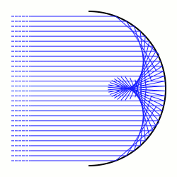
Reflective caustic generated from a circle and parallel rays

In geometrical optics, a caustic is the envelope of a family of light rays. In this picture there is an arc of a circle. The light rays (shown in blue) are coming from a source at infinity, and so arrive parallel. When they hit the circular arc the light rays are scattered in different directions according to the law of reflection. When a light ray hits the arc at a point the light will be reflected as though it had been reflected by the arc's tangent line at that point. The reflected light rays give a one-parameter family of lines in the plane. The envelope of these lines is the reflective caustic. A reflective caustic will generically consist of smooth points and ordinary cusp points.

From the point of view of the calculus of variations, Fermat's principle (in its modern form) implies that light rays are the extremals for the length functional

${\displaystyle L[\gamma ]=\int _{a}^{b}|\gamma '(t)|\,dt}$

among smooth curves ${\displaystyle \gamma }$ on ${\displaystyle [a,b]}$ with fixed endpoints ${\displaystyle \gamma (a)}$ and ${\displaystyle \gamma (b)}$. The caustic determined by a given point ${\displaystyle P}$ (in the image the point is at infinity) is the set of conjugate points to ${\displaystyle P}$. ^[6]

Huygens's principle

Light may pass through anisotropic inhomogeneous media at different rates depending on the direction and starting position of a light ray. The boundary of the set of points to which light can travel from a given point ${\displaystyle q}$ after a time ${\displaystyle t}$ is known as the wave front after time ${\displaystyle t}$, denoted here by ${\displaystyle \Phi _{q}(t)}$. It consists of precisely the points that can be reached from ${\displaystyle q}$ in time ${\displaystyle t}$ by travelling at the speed of light. Huygens's principle asserts that the wave front set ${\displaystyle \Phi _{q_{0}}\!(s+t)}$ is the envelope of the family of wave fronts ${\displaystyle \Phi _{q}(s)}$ for ${\displaystyle q\in \Phi _{q_{0}}(t)}$. More generally, the point ${\displaystyle q_{0}}$ could be replaced by any curve, surface or closed set in space. ^[7]

See also

• Caustic (mathematics)
• Envelope theorem
• Ruled surface

References

1. Bruce, J. W.; Giblin, P. J. (1984), Curves and Singularities, Cambridge University Press, ISBN   0-521-42999-4
2. Eisenhart, Luther P. (2008), A Treatise on the Differential Geometry of Curves and Surfaces, Schwarz Press, ISBN   1-4437-3160-9
3. Forsyth, Andrew Russell (1959), Theory of differential equations, Six volumes bound as three, New York: Dover Publications, MR   0123757 , §§100-106.
4. Evans, Lawrence C. (1998), Partial differential equations, Providence, R.I.: American Mathematical Society, ISBN   978-0-8218-0772-9 .
5. John, Fritz (1991), Partial differential equations (4th ed.), Springer, ISBN   978-0-387-90609-6 .
6. Born, Max (October 1999), Principle of Optics, Cambridge University Press, ISBN   978-0-521-64222-4 , Appendix I: The calculus of variations.
7. Arnold, V. I. (1997), Mathematical Methods of Classical Mechanics, 2nd ed. , Berlin, New York: Springer-Verlag, ISBN   978-0-387-96890-2 , §46.

External links

• Weisstein, Eric W. "Envelope". MathWorld .
• "Envelope of a family of plane curves" at MathCurve.