Simulated annealing (SA) is a probabilistic technique for approximating the global optimum of a given function. Specifically, it is a metaheuristic to approximate global optimization in a large search space for an optimization problem. For large numbers of local optima, SA can find the global optima. It is often used when the search space is discrete. For problems where finding an approximate global optimum is more important than finding a precise local optimum in a fixed amount of time, simulated annealing may be preferable to exact algorithms such as gradient descent or branch and bound.
In mathematical modeling, overfitting is "the production of an analysis that corresponds too closely or exactly to a particular set of data, and may therefore fail to fit to additional data or predict future observations reliably". An overfitted model is a mathematical model that contains more parameters than can be justified by the data. In a mathematical sense, these parameters represent the degree of a polynomial. The essence of overfitting is to have unknowingly extracted some of the residual variation as if that variation represented underlying model structure.

In mathematics, a time series is a series of data points indexed in time order. Most commonly, a time series is a sequence taken at successive equally spaced points in time. Thus it is a sequence of discrete-time data. Examples of time series are heights of ocean tides, counts of sunspots, and the daily closing value of the Dow Jones Industrial Average.

Cross-validation, sometimes called rotation estimation or out-of-sample testing, is any of various similar model validation techniques for assessing how the results of a statistical analysis will generalize to an independent data set. Cross-validation includes resampling and sample splitting methods that use different portions of the data to test and train a model on different iterations. It is often used in settings where the goal is prediction, and one wants to estimate how accurately a predictive model will perform in practice. It can also be used to assess the quality of a fitted model and the stability of its parameters.
Linear trend estimation is a statistical technique used to analyze data patterns. When a series of measurements of a process are treated as a sequence or time series, trend estimation can be used to make and justify statements about tendencies in the data by relating the measurements to the times at which they occurred. This model can then be used to describe the behavior of the observed data.

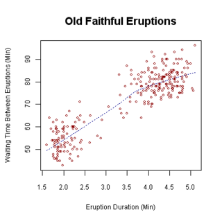
In statistical modeling, regression analysis is a set of statistical processes for estimating the relationships between a dependent variable and one or more independent variables. The most common form of regression analysis is linear regression, in which one finds the line that most closely fits the data according to a specific mathematical criterion. For example, the method of ordinary least squares computes the unique line that minimizes the sum of squared differences between the true data and that line. For specific mathematical reasons, this allows the researcher to estimate the conditional expectation of the dependent variable when the independent variables take on a given set of values. Less common forms of regression use slightly different procedures to estimate alternative location parameters or estimate the conditional expectation across a broader collection of non-linear models.
Random sample consensus (RANSAC) is an iterative method to estimate parameters of a mathematical model from a set of observed data that contains outliers, when outliers are to be accorded no influence on the values of the estimates. Therefore, it also can be interpreted as an outlier detection method. It is a non-deterministic algorithm in the sense that it produces a reasonable result only with a certain probability, with this probability increasing as more iterations are allowed. The algorithm was first published by Fischler and Bolles at SRI International in 1981. They used RANSAC to solve the Location Determination Problem (LDP), where the goal is to determine the points in the space that project onto an image into a set of landmarks with known locations.
Bootstrap aggregating, also called bagging, is a machine learning ensemble meta-algorithm designed to improve the stability and accuracy of machine learning algorithms used in statistical classification and regression. It also reduces variance and helps to avoid overfitting. Although it is usually applied to decision tree methods, it can be used with any type of method. Bagging is a special case of the model averaging approach.
In statistics, resampling is the creation of new samples based on one observed sample. Resampling methods are:
- Permutation tests
- Bootstrapping
- Cross validation
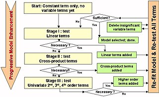
In statistics, stepwise regression is a method of fitting regression models in which the choice of predictive variables is carried out by an automatic procedure. In each step, a variable is considered for addition to or subtraction from the set of explanatory variables based on some prespecified criterion. Usually, this takes the form of a forward, backward, or combined sequence of F-tests or t-tests.

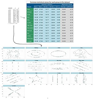
Anscombe's quartet comprises four data sets that have nearly identical simple descriptive statistics, yet have very different distributions and appear very different when graphed. Each dataset consists of eleven (x, y) points. They were constructed in 1973 by the statistician Francis Anscombe to demonstrate both the importance of graphing data when analyzing it, and the effect of outliers and other influential observations on statistical properties. He described the article as being intended to counter the impression among statisticians that "numerical calculations are exact, but graphs are rough".
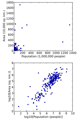
In statistics, data transformation is the application of a deterministic mathematical function to each point in a data set—that is, each data point zi is replaced with the transformed value yi = f(zi), where f is a function. Transforms are usually applied so that the data appear to more closely meet the assumptions of a statistical inference procedure that is to be applied, or to improve the interpretability or appearance of graphs.

Francis John Anscombe was an English statistician.
In statistics, regression validation is the process of deciding whether the numerical results quantifying hypothesized relationships between variables, obtained from regression analysis, are acceptable as descriptions of the data. The validation process can involve analyzing the goodness of fit of the regression, analyzing whether the regression residuals are random, and checking whether the model's predictive performance deteriorates substantially when applied to data that were not used in model estimation.
A plot is a graphical technique for representing a data set, usually as a graph showing the relationship between two or more variables. The plot can be drawn by hand or by a computer. In the past, sometimes mechanical or electronic plotters were used. Graphs are a visual representation of the relationship between variables, which are very useful for humans who can then quickly derive an understanding which may not have come from lists of values. Given a scale or ruler, graphs can also be used to read off the value of an unknown variable plotted as a function of a known one, but this can also be done with data presented in tabular form. Graphs of functions are used in mathematics, sciences, engineering, technology, finance, and other areas.
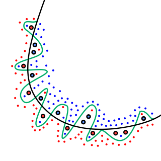
In statistics, an influential observation is an observation for a statistical calculation whose deletion from the dataset would noticeably change the result of the calculation. In particular, in regression analysis an influential observation is one whose deletion has a large effect on the parameter estimates.

Apache Spark is an open-source unified analytics engine for large-scale data processing. Spark provides an interface for programming clusters with implicit data parallelism and fault tolerance. Originally developed at the University of California, Berkeley's AMPLab, the Spark codebase was later donated to the Apache Software Foundation, which has maintained it since.

Symbolic regression (SR) is a type of regression analysis that searches the space of mathematical expressions to find the model that best fits a given dataset, both in terms of accuracy and simplicity.

Alberto Cairo is a Spanish information designer and professor. Cairo is the Knight Chair in Visual Journalism at the School of Communication of the University of Miami.