Autocorrelation, sometimes known as serial correlation in the discrete time case, is the correlation of a signal with a delayed copy of itself as a function of delay. Informally, it is the similarity between observations of a random variable as a function of the time lag between them. The analysis of autocorrelation is a mathematical tool for finding repeating patterns, such as the presence of a periodic signal obscured by noise, or identifying the missing fundamental frequency in a signal implied by its harmonic frequencies. It is often used in signal processing for analyzing functions or series of values, such as time domain signals.

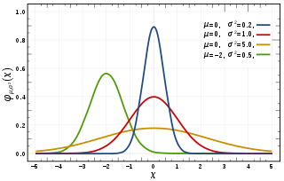
In statistics, a normal distribution or Gaussian distribution is a type of continuous probability distribution for a real-valued random variable. The general form of its probability density function is
In mechanics, the virial theorem provides a general equation that relates the average over time of the total kinetic energy of a stable system of discrete particles, bound by potential forces, with that of the total potential energy of the system. Mathematically, the theorem states

The Allan variance (AVAR), also known as two-sample variance, is a measure of frequency stability in clocks, oscillators and amplifiers. It is named after David W. Allan and expressed mathematically as . The Allan deviation (ADEV), also known as sigma-tau, is the square root of the Allan variance, .
In physics, a Langevin equation is a stochastic differential equation describing how a system evolves when subjected to a combination of deterministic and fluctuating ("random") forces. The dependent variables in a Langevin equation typically are collective (macroscopic) variables changing only slowly in comparison to the other (microscopic) variables of the system. The fast (microscopic) variables are responsible for the stochastic nature of the Langevin equation. One application is to Brownian motion, which models the fluctuating motion of a small particle in a fluid.

In statistical mechanics, the Fokker–Planck equation is a partial differential equation that describes the time evolution of the probability density function of the velocity of a particle under the influence of drag forces and random forces, as in Brownian motion. The equation can be generalized to other observables as well.

In probability theory and statistics, a covariance matrix is a square matrix giving the covariance between each pair of elements of a given random vector. Any covariance matrix is symmetric and positive semi-definite and its main diagonal contains variances.
In mathematics, the moments of a function are certain quantitative measures related to the shape of the function's graph. If the function represents mass density, then the zeroth moment is the total mass, the first moment is the center of mass, and the second moment is the moment of inertia. If the function is a probability distribution, then the first moment is the expected value, the second central moment is the variance, the third standardized moment is the skewness, and the fourth standardized moment is the kurtosis. The mathematical concept is closely related to the concept of moment in physics.
In physics, the S-matrix or scattering matrix relates the initial state and the final state of a physical system undergoing a scattering process. It is used in quantum mechanics, scattering theory and quantum field theory (QFT).

In signal processing, cross-correlation is a measure of similarity of two series as a function of the displacement of one relative to the other. This is also known as a sliding dot product or sliding inner-product. It is commonly used for searching a long signal for a shorter, known feature. It has applications in pattern recognition, single particle analysis, electron tomography, averaging, cryptanalysis, and neurophysiology. The cross-correlation is similar in nature to the convolution of two functions. In an autocorrelation, which is the cross-correlation of a signal with itself, there will always be a peak at a lag of zero, and its size will be the signal energy.
In statistics, econometrics and signal processing, an autoregressive (AR) model is a representation of a type of random process; as such, it is used to describe certain time-varying processes in nature, economics, behavior, etc. The autoregressive model specifies that the output variable depends linearly on its own previous values and on a stochastic term ; thus the model is in the form of a stochastic difference equation. Together with the moving-average (MA) model, it is a special case and key component of the more general autoregressive–moving-average (ARMA) and autoregressive integrated moving average (ARIMA) models of time series, which have a more complicated stochastic structure; it is also a special case of the vector autoregressive model (VAR), which consists of a system of more than one interlocking stochastic difference equation in more than one evolving random variable.

In mathematics, the Ornstein–Uhlenbeck process is a stochastic process with applications in financial mathematics and the physical sciences. Its original application in physics was as a model for the velocity of a massive Brownian particle under the influence of friction. It is named after Leonard Ornstein and George Eugene Uhlenbeck.
In 3-dimensional topology, a part of the mathematical field of geometric topology, the Casson invariant is an integer-valued invariant of oriented integral homology 3-spheres, introduced by Andrew Casson.
In many-body theory, the term Green's function is sometimes used interchangeably with correlation function, but refers specifically to correlators of field operators or creation and annihilation operators.
Resonance fluorescence is the process in which a two-level atom system interacts with the quantum electromagnetic field if the field is driven at a frequency near to the natural frequency of the atom.

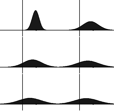
In probability theory and directional statistics, a wrapped normal distribution is a wrapped probability distribution that results from the "wrapping" of the normal distribution around the unit circle. It finds application in the theory of Brownian motion and is a solution to the heat equation for periodic boundary conditions. It is closely approximated by the von Mises distribution, which, due to its mathematical simplicity and tractability, is the most commonly used distribution in directional statistics.
In statistical mechanics, the Griffiths inequality, sometimes also called Griffiths–Kelly–Sherman inequality or GKS inequality, named after Robert B. Griffiths, is a correlation inequality for ferromagnetic spin systems. Informally, it says that in ferromagnetic spin systems, if the 'a-priori distribution' of the spin is invariant under spin flipping, the correlation of any monomial of the spins is non-negative; and the two point correlation of two monomial of the spins is non-negative.
Generalized relative entropy is a measure of dissimilarity between two quantum states. It is a "one-shot" analogue of quantum relative entropy and shares many properties of the latter quantity.
The modified lognormal power-law (MLP) function is a three parameter function that can be used to model data that have characteristics of a log-normal distribution and a power law behavior. It has been used to model the functional form of the initial mass function (IMF). Unlike the other functional forms of the IMF, the MLP is a single function with no joining conditions.
In differential geometry, Santaló's formula describes how to integrate a function on the unit sphere bundle of a Riemannian manifold by first integrating along every geodesic separately and then over the space of all geodesics. It is a standard tool in integral geometry and has applications in isoperimetric and rigidity results. The formula is named after Luis Santaló, who first proved the result in 1952.


