Feasible region

A problem with five linear constraints (in blue, including the non-negativity constraints). In the absence of integer constraints the feasible set is the entire region bounded by blue, but with integer constraints it is the set of red dots.

A closed feasible region of a linear programming problem with three variables is a convex polyhedron.

In mathematical optimization and computer science, a feasible region,feasible set, or solution space is the set of all possible points (sets of values of the choice variables) of an optimization problem that satisfy the problem's constraints, potentially including inequalities, equalities, and integer constraints. ^[1] This is the initial set of candidate solutions to the problem, before the set of candidates has been narrowed down.

For example, consider the problem of minimizing the function ${\displaystyle x^{2}+y^{4}}$ with respect to the variables ${\displaystyle x}$ and ${\displaystyle y,}$ subject to ${\displaystyle 1\leq x\leq 10}$ and ${\displaystyle 5\leq y\leq 12.\,}$ Here the feasible set is the set of pairs (x, y) in which the value of x is at least 1 and at most 10 and the value of y is at least 5 and at most 12. The feasible set of the problem is separate from the objective function, which states the criterion to be optimized and which in the above example is ${\displaystyle x^{2}+y^{4}.}$

In many problems, the feasible set reflects a constraint that one or more variables must be non-negative. In pure integer programming problems, the feasible set is the set of integers (or some subset thereof). In linear programming problems, the feasible set is a convex polytope: a region in multidimensional space whose boundaries are formed by hyperplanes and whose corners are vertices.

Constraint satisfaction is the process of finding a point in the feasible region.

Convex feasible set

See also: Convex optimization

A convex feasible set is one in which a line segment connecting any two feasible points goes through only other feasible points, and not through any points outside the feasible set. Convex feasible sets arise in many types of problems, including linear programming problems, and they are of particular interest because, if the problem has a convex objective function that is to be maximized, it will generally be easier to solve in the presence of a convex feasible set and any local optimum will also be a global optimum.

No feasible set

If the constraints of an optimization problem are mutually contradictory, there are no points that satisfy all the constraints and thus the feasible region is the empty set. In this case the problem has no solution and is said to be infeasible.

Bounded and unbounded feasible sets

A bounded feasible set (top) and an unbounded feasible set (bottom). The set at the bottom continues forever towards the right.

Feasible sets may be bounded or unbounded. For example, the feasible set defined by the constraint set {x ≥ 0, y ≥ 0} is unbounded because in some directions there is no limit on how far one can go and still be in the feasible region. In contrast, the feasible set formed by the constraint set {x ≥ 0, y ≥ 0, x + 2y ≤ 4} is bounded because the extent of movement in any direction is limited by the constraints.

In linear programming problems with n variables, a necessary but insufficient condition for the feasible set to be bounded is that the number of constraints be at least n + 1 (as illustrated by the above example).

If the feasible set is unbounded, there may or may not be an optimum, depending on the specifics of the objective function. For example, if the feasible region is defined by the constraint set {x ≥ 0, y ≥ 0}, then the problem of maximizing x + y has no optimum since any candidate solution can be improved upon by increasing x or y; yet if the problem is to minimizex + y, then there is an optimum (specifically at (x, y) = (0, 0)).

Candidate solution

In optimization and other branches of mathematics, and in search algorithms (a topic in computer science), a candidate solution is a member of the set of possible solutions in the feasible region of a given problem. ^[2] A candidate solution does not have to be a likely or reasonable solution to the problem—it is simply in the set that satisfies all constraints; that is, it is in the set of feasible solutions. Algorithms for solving various types of optimization problems often narrow the set of candidate solutions down to a subset of the feasible solutions, whose points remain as candidate solutions while the other feasible solutions are henceforth excluded as candidates.

The space of all candidate solutions, before any feasible points have been excluded, is called the feasible region, feasible set, search space, or solution space. ^[2] This is the set of all possible solutions that satisfy the problem's constraints. Constraint satisfaction is the process of finding a point in the feasible set.

Genetic algorithm

In the case of the genetic algorithm, the candidate solutions are the individuals in the population being evolved by the algorithm. ^[3]

Calculus

In calculus, an optimal solution is sought using the first derivative test: the first derivative of the function being optimized is equated to zero, and any values of the choice variable(s) that satisfy this equation are viewed as candidate solutions (while those that do not are ruled out as candidates). There are several ways in which a candidate solution might not be an actual solution. First, it might give a minimum when a maximum is being sought (or vice versa), and second, it might give neither a minimum nor a maximum but rather a saddle point or an inflection point, at which a temporary pause in the local rise or fall of the function occurs. Such candidate solutions may be able to be ruled out by use of the second derivative test, the satisfaction of which is sufficient for the candidate solution to be at least locally optimal. Third, a candidate solution may be a local optimum but not a global optimum.

In taking antiderivatives of monomials of the form ${\displaystyle x^{n},}$ the candidate solution using Cavalieri's quadrature formula would be ${\displaystyle {\tfrac {1}{n+1}}x^{n+1}+C.}$ This candidate solution is in fact correct except when ${\displaystyle n=-1.}$

Linear programming

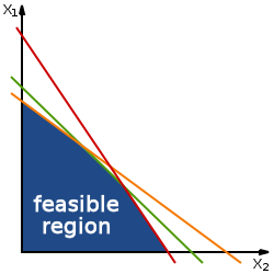
A series of linear programming constraints on two variables produce a region of possible values for those variables. Solvable two-variable problems will have a feasible region in the shape of a convex simple polygon if it is bounded. In an algorithm that tests feasible points sequentially, each tested point is in turn a candidate solution.

In the simplex method for solving linear programming problems, a vertex of the feasible polytope is selected as the initial candidate solution and is tested for optimality; if it is rejected as the optimum, an adjacent vertex is considered as the next candidate solution. This process is continued until a candidate solution is found to be the optimum.

References

1. Beavis, Brian; Dobbs, Ian (1990). Optimisation and Stability Theory for Economic Analysis. New York: Cambridge University Press. p. 32. ISBN   0-521-33605-8.
2. Boyd, Stephen; Vandenberghe, Lieven (2004-03-08). Convex Optimization. Cambridge University Press. ISBN   978-0-521-83378-3.
3. Whitley, Darrell (1994). "A genetic algorithm tutorial" (PDF). Statistics and Computing. 4 (2): 65–85. doi:10.1007/BF00175354. S2CID   3447126.