In mathematical physics and mathematics, the Pauli matrices are a set of three 2 × 2 complex matrices that are traceless, Hermitian, involutory and unitary. Usually indicated by the Greek letter sigma, they are occasionally denoted by tau when used in connection with isospin symmetries.
In statistics, the Gauss–Markov theorem states that the ordinary least squares (OLS) estimator has the lowest sampling variance within the class of linear unbiased estimators, if the errors in the linear regression model are uncorrelated, have equal variances and expectation value of zero. The errors do not need to be normal, nor do they need to be independent and identically distributed. The requirement that the estimator be unbiased cannot be dropped, since biased estimators exist with lower variance. See, for example, the James–Stein estimator, ridge regression, or simply any degenerate estimator.

In statistical modeling, regression analysis is a set of statistical processes for estimating the relationships between a dependent variable and one or more error-free independent variables. The most common form of regression analysis is linear regression, in which one finds the line that most closely fits the data according to a specific mathematical criterion. For example, the method of ordinary least squares computes the unique line that minimizes the sum of squared differences between the true data and that line. For specific mathematical reasons, this allows the researcher to estimate the conditional expectation of the dependent variable when the independent variables take on a given set of values. Less common forms of regression use slightly different procedures to estimate alternative location parameters or estimate the conditional expectation across a broader collection of non-linear models.
In statistics, econometrics, epidemiology and related disciplines, the method of instrumental variables (IV) is used to estimate causal relationships when controlled experiments are not feasible or when a treatment is not successfully delivered to every unit in a randomized experiment. Intuitively, IVs are used when an explanatory variable of interest is correlated with the error term (endogenous), in which case ordinary least squares and ANOVA give biased results. A valid instrument induces changes in the explanatory variable but has no independent effect on the dependent variable and is not correlated with the error term, allowing a researcher to uncover the causal effect of the explanatory variable on the dependent variable.
In statistics, omitted-variable bias (OVB) occurs when a statistical model leaves out one or more relevant variables. The bias results in the model attributing the effect of the missing variables to those that were included.
In statistics, the theory of minimum norm quadratic unbiased estimation (MINQUE) was developed by C. R. Rao. MINQUE is a theory alongside other estimation methods in estimation theory, such as the method of moments or maximum likelihood estimation. Similar to the theory of best linear unbiased estimation, MINQUE is specifically concerned with linear regression models. The method was originally conceived to estimate heteroscedastic error variance in multiple linear regression. MINQUE estimators also provide an alternative to maximum likelihood estimators or restricted maximum likelihood estimators for variance components in mixed effects models. MINQUE estimators are quadratic forms of the response variable and are used to estimate a linear function of the variances.

In statistics, ordinary least squares (OLS) is a type of linear least squares method for choosing the unknown parameters in a linear regression model by the principle of least squares: minimizing the sum of the squares of the differences between the observed dependent variable in the input dataset and the output of the (linear) function of the independent variable. Some sources consider OLS to be linear regression.

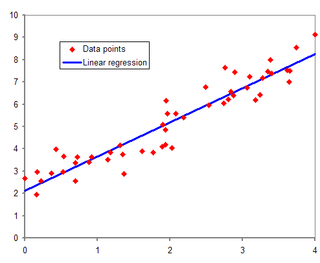
In statistics, simple linear regression (SLR) is a linear regression model with a single explanatory variable. That is, it concerns two-dimensional sample points with one independent variable and one dependent variable and finds a linear function that, as accurately as possible, predicts the dependent variable values as a function of the independent variable. The adjective simple refers to the fact that the outcome variable is related to a single predictor.
Difference in differences is a statistical technique used in econometrics and quantitative research in the social sciences that attempts to mimic an experimental research design using observational study data, by studying the differential effect of a treatment on a 'treatment group' versus a 'control group' in a natural experiment. It calculates the effect of a treatment on an outcome by comparing the average change over time in the outcome variable for the treatment group to the average change over time for the control group. Although it is intended to mitigate the effects of extraneous factors and selection bias, depending on how the treatment group is chosen, this method may still be subject to certain biases.
In statistics, a fixed effects model is a statistical model in which the model parameters are fixed or non-random quantities. This is in contrast to random effects models and mixed models in which all or some of the model parameters are random variables. In many applications including econometrics and biostatistics a fixed effects model refers to a regression model in which the group means are fixed (non-random) as opposed to a random effects model in which the group means are a random sample from a population. Generally, data can be grouped according to several observed factors. The group means could be modeled as fixed or random effects for each grouping. In a fixed effects model each group mean is a group-specific fixed quantity.
In statistics, generalized least squares (GLS) is a method used to estimate the unknown parameters in a linear regression model. It is used when there is a non-zero amount of correlation between the residuals in the regression model. GLS is employed to improve statistical efficiency and reduce the risk of drawing erroneous inferences, as compared to conventional least squares and weighted least squares methods. It was first described by Alexander Aitken in 1935.
In estimation theory and decision theory, a Bayes estimator or a Bayes action is an estimator or decision rule that minimizes the posterior expected value of a loss function. Equivalently, it maximizes the posterior expectation of a utility function. An alternative way of formulating an estimator within Bayesian statistics is maximum a posteriori estimation.
The topic of heteroskedasticity-consistent (HC) standard errors arises in statistics and econometrics in the context of linear regression and time series analysis. These are also known as heteroskedasticity-robust standard errors, Eicker–Huber–White standard errors, to recognize the contributions of Friedhelm Eicker, Peter J. Huber, and Halbert White.
In statistics, principal component regression (PCR) is a regression analysis technique that is based on principal component analysis (PCA). PCR is a form of reduced rank regression. More specifically, PCR is used for estimating the unknown regression coefficients in a standard linear regression model.
In statistical theory, the field of high-dimensional statistics studies data whose dimension is larger than typically considered in classical multivariate analysis. The area arose owing to the emergence of many modern data sets in which the dimension of the data vectors may be comparable to, or even larger than, the sample size, so that justification for the use of traditional techniques, often based on asymptotic arguments with the dimension held fixed as the sample size increased, was lacking.
The purpose of this page is to provide supplementary materials for the ordinary least squares article, reducing the load of the main article with mathematics and improving its accessibility, while at the same time retaining the completeness of exposition.

In statistics, errors-in-variables models or measurement error models are regression models that account for measurement errors in the independent variables. In contrast, standard regression models assume that those regressors have been measured exactly, or observed without error; as such, those models account only for errors in the dependent variables, or responses.
In econometrics, the Arellano–Bond estimator is a generalized method of moments estimator used to estimate dynamic models of panel data. It was proposed in 1991 by Manuel Arellano and Stephen Bond, based on the earlier work by Alok Bhargava and John Denis Sargan in 1983, for addressing certain endogeneity problems. The GMM-SYS estimator is a system that contains both the levels and the first difference equations. It provides an alternative to the standard first difference GMM estimator.
A partially linear model is a form of semiparametric model, since it contains parametric and nonparametric elements. Application of the least squares estimators is available to partially linear model, if the hypothesis of the known of nonparametric element is valid. Partially linear equations were first used in the analysis of the relationship between temperature and usage of electricity by Engle, Granger, Rice and Weiss (1986). Typical application of partially linear model in the field of Microeconomics is presented by Tripathi in the case of profitability of firm's production in 1997. Also, partially linear model applied successfully in some other academic field. In 1994, Zeger and Diggle introduced partially linear model into biometrics. In environmental science, Parda-Sanchez et al. used partially linear model to analysis collected data in 2000. So far, partially linear model was optimized in many other statistic methods. In 1988, Robinson applied Nadaraya-Waston kernel estimator to test the nonparametric element to build a least-squares estimator After that, in 1997, local linear method was found by Truong.
In statistics, the Innovation Method provides an estimator for the parameters of stochastic differential equations given a time series of observations of the state variables. In the framework of continuous-discrete state space models, the innovation estimator is obtained by maximizing the log-likelihood of the corresponding discrete-time innovation process with respect to the parameters. The innovation estimator can be classified as a M-estimator, a quasi-maximum likelihood estimator or a prediction error estimator depending on the inferential considerations that want to be emphasized. The innovation method is a system identification technique for developing mathematical models of dynamical systems from measured data and for the optimal design of experiments.


