Method of averaging

Last updated

In mathematics, more specifically in dynamical systems, the method of averaging (also called averaging theory) exploits systems containing time-scales separation: a fast oscillationversus a slow drift. It suggests that we perform an averaging over a given amount of time in order to iron out the fast oscillations and observe the qualitative behavior from the resulting dynamics. The approximated solution holds under finite time inversely proportional to the parameter denoting the slow time scale. It turns out to be a customary problem where there exists the trade off between how good is the approximated solution balanced by how much time it holds to be close to the original solution.

Contents

More precisely, the system has the following form

of a phase space variable The fast oscillation is given by versus a slow drift of . The averaging method yields an autonomous dynamical system

which approximates the solution curves of inside a connected and compact region of the phase space and over time of .

Under the validity of this averaging technique, the asymptotic behavior of the original system is captured by the dynamical equation for . In this way, qualitative methods for autonomous dynamical systems may be employed to analyze the equilibria and more complex structures, such as slow manifold and invariant manifolds, as well as their stability in the phase space of the averaged system.

In addition, in a physical application it might be reasonable or natural to replace a mathematical model, which is given in the form of the differential equation for , with the corresponding averaged system , in order to use the averaged system to make a prediction and then test the prediction against the results of a physical experiment. [1]

The averaging method has a long history, which is deeply rooted in perturbation problems that arose in celestial mechanics (see, for example in [2] ).

First example

Figure 1: Solution to perturbed logistic growth equation
x
.
=
e
(
x
(
1
-
x
)
+
sin
[?]
t
)
x
[?]
R
,
e
=
0.05
{\displaystyle {\dot {x}}=\varepsilon (x(1-x)+\sin {t})~x\in \mathbb {R} ,~\varepsilon =0.05}
(blue solid line) and the averaged equation
y
.
=
e
y
(
1
-
y
)
,
y
[?]
R
{\displaystyle {\dot {y}}=\varepsilon y(1-y),~y\in \mathbb {R} }
(orange solid line). Logistic growth equation.png
Figure 1: Solution to perturbed logistic growth equation (blue solid line) and the averaged equation   (orange solid line).

Consider a perturbed logistic growth

and the averaged equation

The purpose of the method of averaging is to tell us the qualitative behavior of the vector field when we average it over a period of time. It guarantees that the solution approximates for times Exceptionally: in this example the approximation is even better, it is valid for all times. We present it in a section below.

Definitions

We assume the vector field to be of differentiability class with (or even we will only say smooth), which we will denote . We expand this time-dependent vector field in a Taylor series (in powers of ) with remainder . We introduce the following notation: [2]

where is the -th derivative with . As we are concerned with averaging problems, in general is zero, so it turns out that we will be interested in vector fields given by

Besides, we define the following initial value problem to be in the standard form: [2]

Theorem: averaging in the periodic case

Consider for every connected and bounded and every there exist and such that the original system (a non-autonomous dynamical system) given by

has solution , where is periodic with period and Failed to parse (SVG (MathML can be enabled via browser plugin): Invalid response ("Math extension cannot connect to Restbase.") from server "http://localhost:6011/en.wikipedia.org/v1/":): {\displaystyle f^{[2]} \in C^r(D \times \R \times \R^+; \R^n)} both with bounded on bounded sets. Then there exists a constant such that the solution of the averagedsystem (autonomous dynamical system) is

is

for and .

Remarks

Strategy of the proof

Krylov-Bogoliubov realized that the slow dynamics of the system determines the leading order of the asymptotic solution.

In order to proof it, they proposed a near-identity transformation, which turned out to be a change of coordinates with its own time-scale transforming the original system to the averaged one.

Sketch of the proof

  1. Determination of a near-identity transformation: the smooth mapping where is assumed to be regular enough and periodic. The proposed change of coordinates is given by .
  2. Choose an appropriate solving the homological equation of the averaging theory: .
  3. Change of coordinates carries the original system to
  4. Estimation of error due to truncation and comparison to the original variable.

Non-autonomous class of systems: more examples

Along the history of the averaging technique, there is class of system extensively studied which give us meaningful examples we will discuss below. The class of system is given by:

where is smooth. This system is similar to a linear system with a small nonlinear perturbation given by :

differing from the standard form. Hence there is a necessity to perform a transformation to make it in the standard form explicitly. [2] We are able to change coordinates using variation of constants method. We look at the unperturbed system, i.e. , given by

which has the fundamental solution corresponding to a rotation. Then the time-dependent change of coordinates is where is the coordinates respective to the standard form.

If we take the time derivative in both sides and invert the fundamental matrix we obtain

Remarks

If we may apply averaging so long as a neighborhood of the origin is excluded (since the polar coordinates fail):

where the averaged system is

Example: Misleading averaging results

Figure 2: A simple harmonic oscillator with small periodic damping term given by
z
"
+
4
e
cos
2
[?]
(
t
)
z
.
+
z
=
0
,
z
(
0
)
=
0
,
z
.
(
0
)
=
1
;
e
=
0.05
{\displaystyle {\ddot {z}}+4\varepsilon \cos ^{2}{(t)}{\dot {z}}+z=0,~z(0)=0,~{\dot {z}}(0)=1;~\varepsilon =0.05}
.The numerical simulation of the original equation (blue solid line) is compared with averaging system (orange dashed line) and the crude averaged system (green dash-dotted line). The left plot displays the solution evolved in time and the right plot represents on the phase space. We note that the crude averaging disagrees with the expected solution. Averaging example Crude averaging z axis.png
Figure 2: A simple harmonic oscillator with small periodic damping term given by .The numerical simulation of the original equation (blue solid line) is compared with averaging system (orange dashed line) and the crude averaged system (green dash-dotted line). The left plot displays the solution evolved in time and the right plot represents on the phase space. We note that the crude averaging disagrees with the expected solution.

The method contains some assumptions and restrictions. These limitations play important role when we average the original equation which is not into the standard form, and we can discuss counterexample of it. The following example in order to discourage this hurried averaging: [2]

where we put following the previous notation.

This systems corresponds to a damped harmonic oscillator where the damping term oscillates between and . Averaging the friction term over one cycle of yields the equation:

The solution is

which the convergence rate to the origin is . The averaged system obtained from the standard form yields:

which in the rectangular coordinate shows explicitly that indeed the rate of convergence to the origin is differing from the previous crude averaged system:

Example: Van der Pol Equation

Figure 3: Phase space of a Van der Pol oscillator with
e
=
0.1
{\displaystyle \varepsilon =0.1}
. The stable limit cycle (orange solid line) in the system is captured correctly by the qualitative analysis of the averaged system. For two different initial conditions ( black dots ) we observe the trajectories.(dashed blue line) converging to the periodic orbit. Van der pol qualitative.png
Figure 3: Phase space of a Van der Pol oscillator with . The stable limit cycle (orange solid line) in the system is captured correctly by the qualitative analysis of the averaged system. For two different initial conditions ( black dots ) we observe the trajectories.(dashed blue line) converging to the periodic orbit.

Van der Pol was concerned with obtaining approximate solutions for equations of the type

where following the previous notation. This system is often called the Van der Pol oscillator. Applying periodic averaging to this nonlinear oscillator provides qualitative knowledge of the phase space without solving the system explicitly.

The averaged system is

and we can analyze the fixed points and their stability. There is an unstable fixed point at the origin and a stable limit cycle represented by .

The existence of such stable limit-cycle can be stated as a theorem.

Theorem (Existence of a periodic orbit) [5] : If is a hyperbolic fixed point of

Then there exists such that for all ,

has a unique hyperbolic periodic orbit of the same stability type as .

The proof can be found at Guckenheimer and Holmes, [5] Sanders et al. [2] and for the angle case in Chicone. [1]

Example: Restricting the time interval

Figure 4: The plot depicts two fundamental quantities the average technique is based on: the bounded and connected region
D
{\displaystyle D}
of the phase space and how long (defined by the constant
c
{\displaystyle c}
) the averaged solution is valid. For this case,
z
"
+
z
=
8
e
cos
[?]
(
t
)
z
.
2
,
z
(
0
)
=
0
,
z
.
(
0
)
=
1
;
8
e
=
2
15
{\textstyle {\ddot {z}}+z=8\varepsilon \cos {(t)}{\dot {z}}^{2},~z(0)=0,~{\dot {z}}(0)=1;~8\varepsilon ={\frac {2}{15}}}
. Note that both solutions blow up in finite time.  Hence,
D
{\displaystyle D}
has been chosen accordingly in order to maintain the boundedness of the solution and the time interval of validity of the approximation is
0
<=
e
t
<
L
<
1
3
{\displaystyle 0\leq \varepsilon t<L<{\frac {1}{3}}}
. Restricting time scale.png
Figure 4: The plot depicts two fundamental quantities the average technique is based on: the bounded and connected region of the phase space and how long (defined by the constant ) the averaged solution is valid. For this case, . Note that both solutions blow up in finite time.  Hence, has been chosen accordingly in order to maintain the boundedness of the solution and the time interval of validity of the approximation is .

The average theorem assumes existence of a connected and bounded region which affects the time interval of the result validity. The following example points it out. Consider the

where . The averaged system consists of

which under this initial condition indicates that the original solution behaves like

where it holds on a bounded region over .

Damped Pendulum

Consider a damped pendulum whose point of suspension is vibrated vertically by a small amplitude, high frequency signal (this is usually known as dithering ). The equation of motion for such a pendulum is given by

where describes the motion of the suspension point, describes the damping of the pendulum, and is the angle made by the pendulum with the vertical.

The phase space form of this equation is given by

where we have introduced the variable and written the system as an autonomous, first-order system in -space.

Suppose that the angular frequency of the vertical vibrations, , is much greater than the natural frequency of the pendulum, . Suppose also that the amplitude of the vertical vibrations, , is much less than the length of the pendulum. The pendulum's trajectory in phase space will trace out a spiral around a curve , moving along at the slow rate but moving around it at the fast rate . The radius of the spiral around will be small and proportional to . The average behaviour of the trajectory, over a timescale much larger than , will be to follow the curve .

Extension error estimates

Average technique for initial value problems has been treated up to now with an validity error estimates of order . However, there are circumstances where the estimates can be extended for further times, even the case for all times. [2] Below we deal with a system containing an asymptotically stable fixed point. Such situation recapitulates what is illustrated in Figure 1.

Theorem (Eckhaus [6] /Sanchez-Palencia [7] ) Consider the initial value problem

Suppose

exists and contains an asymptotically stable fixed point in the linear approximation. Moreover, is continuously differentiable with respect to in and has a domain of attraction . For any compact and for all

with in the general case and in the periodic case.

Related Research Articles

<span class="mw-page-title-main">Pauli matrices</span> Matrices important in quantum mechanics and the study of spin

In mathematical physics and mathematics, the Pauli matrices are a set of three 2 × 2 complex matrices which are Hermitian, involutory and unitary. Usually indicated by the Greek letter sigma, they are occasionally denoted by tau when used in connection with isospin symmetries.

<span class="mw-page-title-main">Astronomical coordinate systems</span> System for specifying positions of celestial objects

Astronomicalcoordinate systems are organized arrangements for specifying positions of satellites, planets, stars, galaxies, and other celestial objects relative to physical reference points available to a situated observer. Coordinate systems in astronomy can specify an object's position in three-dimensional space or plot merely its direction on a celestial sphere, if the object's distance is unknown or trivial.

<span class="mw-page-title-main">Unit vector</span> Vector of length one

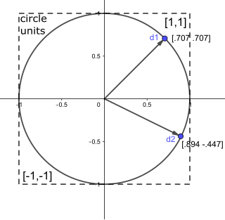
In mathematics, a unit vector in a normed vector space is a vector of length 1. A unit vector is often denoted by a lowercase letter with a circumflex, or "hat", as in .

In mechanics and geometry, the 3D rotation group, often denoted SO(3), is the group of all rotations about the origin of three-dimensional Euclidean space under the operation of composition.

<span class="mw-page-title-main">Laplace operator</span> Differential operator

In mathematics, the Laplace operator or Laplacian is a differential operator given by the divergence of the gradient of a scalar function on Euclidean space. It is usually denoted by the symbols , (where is the nabla operator), or . In a Cartesian coordinate system, the Laplacian is given by the sum of second partial derivatives of the function with respect to each independent variable. In other coordinate systems, such as cylindrical and spherical coordinates, the Laplacian also has a useful form. Informally, the Laplacian Δf (p) of a function f at a point p measures by how much the average value of f over small spheres or balls centered at p deviates from f (p).

In continuum mechanics, the infinitesimal strain theory is a mathematical approach to the description of the deformation of a solid body in which the displacements of the material particles are assumed to be much smaller than any relevant dimension of the body; so that its geometry and the constitutive properties of the material at each point of space can be assumed to be unchanged by the deformation.

Linear elasticity is a mathematical model of how solid objects deform and become internally stressed due to prescribed loading conditions. It is a simplification of the more general nonlinear theory of elasticity and a branch of continuum mechanics.

In probability theory, the Borel–Kolmogorov paradox is a paradox relating to conditional probability with respect to an event of probability zero. It is named after Émile Borel and Andrey Kolmogorov.

<span class="mw-page-title-main">Vector fields in cylindrical and spherical coordinates</span> Vector field representation in 3D curvilinear coordinate systems

Note: This page uses common physics notation for spherical coordinates, in which is the angle between the z axis and the radius vector connecting the origin to the point in question, while is the angle between the projection of the radius vector onto the x-y plane and the x axis. Several other definitions are in use, and so care must be taken in comparing different sources.

<span class="mw-page-title-main">Hamilton–Jacobi equation</span> A reformulation of Newtons laws of motion using the calculus of variations

In physics, the Hamilton–Jacobi equation, named after William Rowan Hamilton and Carl Gustav Jacob Jacobi, is an alternative formulation of classical mechanics, equivalent to other formulations such as Newton's laws of motion, Lagrangian mechanics and Hamiltonian mechanics.

<span class="mw-page-title-main">Torus knot</span> Knot which lies on the surface of a torus in 3-dimensional space

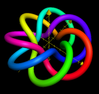
In knot theory, a torus knot is a special kind of knot that lies on the surface of an unknotted torus in R3. Similarly, a torus link is a link which lies on the surface of a torus in the same way. Each torus knot is specified by a pair of coprime integers p and q. A torus link arises if p and q are not coprime. A torus knot is trivial if and only if either p or q is equal to 1 or −1. The simplest nontrivial example is the (2,3)-torus knot, also known as the trefoil knot.

In mathematical analysis, and applications in geometry, applied mathematics, engineering, and natural sciences, a function of a real variable is a function whose domain is the real numbers , or a subset of that contains an interval of positive length. Most real functions that are considered and studied are differentiable in some interval. The most widely considered such functions are the real functions, which are the real-valued functions of a real variable, that is, the functions of a real variable whose codomain is the set of real numbers.

In statistics, econometrics, and signal processing, an autoregressive (AR) model is a representation of a type of random process; as such, it is used to describe certain time-varying processes in nature, economics, behavior, etc. The autoregressive model specifies that the output variable depends linearly on its own previous values and on a stochastic term ; thus the model is in the form of a stochastic difference equation. Together with the moving-average (MA) model, it is a special case and key component of the more general autoregressive–moving-average (ARMA) and autoregressive integrated moving average (ARIMA) models of time series, which have a more complicated stochastic structure; it is also a special case of the vector autoregressive model (VAR), which consists of a system of more than one interlocking stochastic difference equation in more than one evolving random variable.

A parametric surface is a surface in the Euclidean space which is defined by a parametric equation with two parameters . Parametric representation is a very general way to specify a surface, as well as implicit representation. Surfaces that occur in two of the main theorems of vector calculus, Stokes' theorem and the divergence theorem, are frequently given in a parametric form. The curvature and arc length of curves on the surface, surface area, differential geometric invariants such as the first and second fundamental forms, Gaussian, mean, and principal curvatures can all be computed from a given parametrization.

<span class="mw-page-title-main">Voigt effect</span>

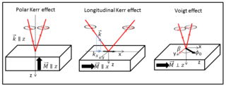
The Voigt effect is a magneto-optical phenomenon which rotates and elliptizes linearly polarised light sent into an optically active medium. Unlike many other magneto-optical effects such as the Kerr or Faraday effect which are linearly proportional to the magnetization, the Voigt effect is proportional to the square of the magnetization and can be seen experimentally at normal incidence. There are several denominations for this effect in the literature: the Cotton–Mouton effect, the Voigt effect, and magnetic-linear birefringence. This last denomination is closer in the physical sense, where the Voigt effect is a magnetic birefringence of the material with an index of refraction parallel and perpendicular ) to the magnetization vector or to the applied magnetic field.

<span class="mw-page-title-main">Dual quaternion</span>

In mathematics, the dual quaternions are an 8-dimensional real algebra isomorphic to the tensor product of the quaternions and the dual numbers. Thus, they may be constructed in the same way as the quaternions, except using dual numbers instead of real numbers as coefficients. A dual quaternion can be represented in the form A + εB, where A and B are ordinary quaternions and ε is the dual unit, which satisfies ε2 = 0 and commutes with every element of the algebra. Unlike quaternions, the dual quaternions do not form a division algebra.

The Krylov–Bogolyubov averaging method is a mathematical method for approximate analysis of oscillating processes in non-linear mechanics. The method is based on the averaging principle when the exact differential equation of the motion is replaced by its averaged version. The method is named after Nikolay Krylov and Nikolay Bogoliubov.

In mathematical analysis and its applications, a function of several real variables or real multivariate function is a function with more than one argument, with all arguments being real variables. This concept extends the idea of a function of a real variable to several variables. The "input" variables take real values, while the "output", also called the "value of the function", may be real or complex. However, the study of the complex-valued functions may be easily reduced to the study of the real-valued functions, by considering the real and imaginary parts of the complex function; therefore, unless explicitly specified, only real-valued functions will be considered in this article.

The Clohessy–Wiltshire equations describe a simplified model of orbital relative motion, in which the target is in a circular orbit, and the chaser spacecraft is in an elliptical or circular orbit. This model gives a first-order approximation of the chaser's motion in a target-centered coordinate system. It is used to plan the rendezvous of the chaser with the target.

<span class="mw-page-title-main">Calculus on Euclidean space</span>

In mathematics, calculus on Euclidean space is a generalization of calculus of functions in one or several variables to calculus of functions on Euclidean space as well as a finite-dimensional real vector space. This calculus is also known as advanced calculus, especially in the United States. It is similar to multivariable calculus but is somehow more sophisticated in that it uses linear algebra more extensively and covers some concepts from differential geometry such as differential forms and Stokes' formula in terms of differential forms. This extensive use of linear algebra also allows a natural generalization of multivariable calculus to calculus on Banach spaces or topological vector spaces.

References

  1. 1 2 3 Charles., Chicone, Carmen (2006). Ordinary differential equations with applications (2nd ed.). New York: Springer. ISBN   9780387307695. OCLC   288193020.{{cite book}}: CS1 maint: multiple names: authors list (link)
  2. 1 2 3 4 5 6 7 8 9 10 Sanders, Jan A.; Verhulst, Ferdinand; Murdock, James (2007). Averaging Methods in Nonlinear Dynamical Systems. Applied Mathematical Sciences. Vol. 59. doi:10.1007/978-0-387-48918-6. ISBN   978-0-387-48916-2.
  3. Murdock, James A. (1999). Perturbations : theory and methods. Philadelphia: Society for Industrial and Applied Mathematics. ISBN   978-0898714432. OCLC   41612407.
  4. Hale, Jack K. (1980). Ordinary differential equations (2nd ed.). Huntington, N.Y.: R.E. Krieger Pub. Co. ISBN   978-0898740110. OCLC   5170595.
  5. 1 2 Guckenheimer, John; Holmes, Philip (1983). Nonlinear Oscillations, Dynamical Systems, and Bifurcations of Vector Fields. Applied Mathematical Sciences. Vol. 42. doi:10.1007/978-1-4612-1140-2. ISBN   978-1-4612-7020-1. ISSN   0066-5452.
  6. Eckhaus, Wiktor (1975-03-01). "New approach to the asymptotic theory of nonlinear oscillations and wave-propagation". Journal of Mathematical Analysis and Applications. 49 (3): 575–611. doi: 10.1016/0022-247X(75)90200-0 . ISSN   0022-247X.
  7. Sanchez-Palencia, Enrique (1976-01-01). "Methode de centrage-estimation de l'erreur et comportement des trajectoires dans l'espace des phases". International Journal of Non-Linear Mechanics. 11 (4): 251–263. Bibcode:1976IJNLM..11..251S. doi:10.1016/0020-7462(76)90004-4. ISSN   0020-7462.