Montgomery curve

Last updated September 11, 2024

In mathematics, the Montgomery curve is a form of elliptic curve introduced by Peter L. Montgomery in 1987,^[1] different from the usual Weierstrass form. It is used for certain computations, and in particular in different cryptography applications.

Definition

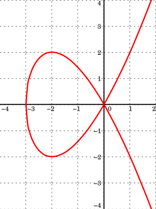
A Montgomery curve over a field $K$ is defined by the equation

M_{A,B}:By^{2}=x^{3}+Ax^{2}+x

for certain $A, B \in K$ and with $B (A 2 - 4) \neq 0$ .

Generally this curve is considered over a finite field K (for example, over a finite field of $q$ elements, $K = F q$ ) with characteristic different from 2 and with $A \neq \pm2$ and $B \neq 0$ , but they are also considered over the rationals with the same restrictions for $A$ and $B$ .

Montgomery arithmetic

It is possible to do some "operations" between the points of an elliptic curve: "adding" two points $P,Q$ consists of finding a third one $R$ such that $R=P+Q$ ; "doubling" a point consists of computing $[2]P=P+P$ (For more information about operations see The group law) and below.

A point $P=(x,y)$ on the elliptic curve in the Montgomery form $By^{2}=x^{3}+Ax^{2}+x$ can be represented in Montgomery coordinates $P=(X:Z)$ , where $P=(X:Z)$ are projective coordinates and $x=X/Z$ for $Z\neq 0$ .

Notice that this kind of representation for a point loses information: indeed, in this case, there is no distinction between the affine points $(x,y)$ and $(x,-y)$ because they are both given by the point $(X:Z)$ . However, with this representation it is possible to obtain multiples of points, that is, given $P=(X:Z)$ , to compute $[n]P=(X_{n}:Z_{n})$ .

Now, considering the two points $P_{n}=[n]P=(X_{n}:Z_{n})$ and $P_{m}=[m]P=(X_{m}:Z_{m})$ : their sum is given by the point $P_{m+n}=P_{m}+P_{n}=(X_{m+n}:Z_{m+n})$ whose coordinates are:

X_{m+n}=Z_{m-n}((X_{m}-Z_{m})(X_{n}+Z_{n})+(X_{m}+Z_{m})(X_{n}-Z_{n}))^{2}

Z_{m+n}=X_{m-n}((X_{m}-Z_{m})(X_{n}+Z_{n})-(X_{m}+Z_{m})(X_{n}-Z_{n}))^{2}

If $m=n$ , then the operation becomes a "doubling"; the coordinates of $[2]P_{n}=P_{n}+P_{n}=P_{2n}=(X_{2n}:Z_{2n})$ are given by the following equations:

4X_{n}Z_{n}=(X_{n}+Z_{n})^{2}-(X_{n}-Z_{n})^{2}

X_{2n}=(X_{n}+Z_{n})^{2}(X_{n}-Z_{n})^{2}

Z_{2n}=(4X_{n}Z_{n})((X_{n}-Z_{n})^{2}+((A+2)/4)(4X_{n}Z_{n}))

The first operation considered above (addition) has a time-cost of 3M+2S, where M denotes the multiplication between two general elements of the field on which the elliptic curve is defined, while S denotes squaring of a general element of the field.

The second operation (doubling) has a time-cost of 2M + 2S + 1D, where D denotes the multiplication of a general element by a constant; notice that the constant is $(A+2)/4$ , so $A$ can be chosen in order to have a small D.

Algorithm and example

The following algorithm represents a doubling of a point $P_{1}=(X_{1}:Z_{1})$ on an elliptic curve in the Montgomery form.

It is assumed that $Z_{1}=1$ . The cost of this implementation is 1M + 2S + 1*A + 3add + 1*4. Here M denotes the multiplications required, S indicates the squarings, and a refers to the multiplication by A.

XX_{1}=X_{1}^{2}\,

X_{2}=(XX_{1}-1)^{2}\,

Z_{2}=4X_{1}(XX_{1}+aX_{1}+1)\,

Example

Let $P_{1}=(2,{\sqrt {3}})$ be a point on the curve $2y^{2}=x^{3}-x^{2}+x$ . In coordinates $(X_{1}:Z_{1})$ , with $x_{1}=X_{1}/Z_{1}$ , $P_{1}=(2:1)$ .

Then:

XX_{1}=X_{1}^{2}=4\,

X_{2}=(XX_{1}-1)^{2}=9\,

Z_{2}=4X_{1}(XX_{1}+AX_{1}+1)=24\,

The result is the point $P_{2}=(X_{2}:Z_{2})=(9:24)$ such that $P_{2}=2P_{1}$ .

Addition

Given two points $P_{1}=(x_{1},y_{1})$ , $P_{2}=(x_{2},y_{2})$ on the Montgomery curve $M_{A,B}$ in affine coordinates, the point $P_{3}=P_{1}+P_{2}$ represents, geometrically the third point of intersection between $M_{A,B}$ and the line passing through $P_{1}$ and $P_{2}$ . It is possible to find the coordinates $(x_{3},y_{3})$ of $P_{3}$ , in the following way:

1) consider a generic line $~y=lx+m$ in the affine plane and let it pass through $P_{1}$ and $P_{2}$ (impose the condition), in this way, one obtains $l={\frac {y_{2}-y_{1}}{x_{2}-x_{1}}}$ and $m=y_{1}-\left({\frac {y_{2}-y_{1}}{x_{2}-x_{1}}}\right)x_{1}$ ;

2) intersect the line with the curve $M_{A,B}$ , substituting the $~y$ variable in the curve equation with $~y=lx+m$ ; the following equation of third degree is obtained:

x^{3}+(A-Bl^{2})x^{2}+(1-2Blm)x-Bm^{2}=0.

As it has been observed before, this equation has three solutions that correspond to the $~x$ coordinates of $P_{1}$ , $P_{2}$ and $P_{3}$ . In particular this equation can be re-written as:

(x-x_{1})(x-x_{2})(x-x_{3})=0

3) Comparing the coefficients of the two identical equations given above, in particular the coefficients of the terms of second degree, one gets:

-x_{1}-x_{2}-x_{3}=A-Bl^{2}

.

So, $x_{3}$ can be written in terms of $x_{1}$ , $y_{1}$ , $x_{2}$ , $y_{2}$ , as:

x_{3}=B\left({\frac {y_{2}-y_{1}}{x_{2}-x_{1}}}\right)^{2}-A-x_{1}-x_{2}.

4) To find the $~y$ coordinate of the point $P_{3}$ it is sufficient to substitute the value $x_{3}$ in the line $~y=lx+m$ . Notice that this will not give the point $P_{3}$ directly. Indeed, with this method one find the coordinates of the point $~R$ such that $R+P_{1}+P_{2}=P_{\infty }$ , but if one needs the resulting point of the sum between $P_{1}$ and $P_{2}$ , then it is necessary to observe that: $R+P_{1}+P_{2}=P_{\infty }$ if and only if $-R=P_{1}+P_{2}$ . So, given the point $~R$ , it is necessary to find $~-R$ , but this can be done easily by changing the sign to the $~y$ coordinate of $~R$ . In other words, it will be necessary to change the sign of the $~y$ coordinate obtained by substituting the value $x_{3}$ in the equation of the line.

Resuming, the coordinates of the point $P_{3}=(x_{3},y_{3})$ , $P_{3}=P_{1}+P_{2}$ are:

x_{3}={\frac {B(y_{2}-y_{1})^{2}}{(x_{2}-x_{1})^{2}}}-A-x_{1}-x_{2}

y_{3}={\frac {(2x_{1}+x_{2}+A)(y_{2}-y_{1})}{x_{2}-x_{1}}}-{\frac {B(y_{2}-y_{1})^{3}}{(x_{2}-x_{1})^{3}}}-y_{1}

Doubling

Given a point $P_{1}$ on the Montgomery curve $M_{A,B}$ , the point $[2]P_{1}$ represents geometrically the third point of intersection between the curve and the line tangent to $P_{1}$ ; so, to find the coordinates of the point $P_{3}=2P_{1}$ it is sufficient to follow the same method given in the addition formula; however, in this case, the line y = lx + m has to be tangent to the curve at $P_{1}$ , so, if $M_{A,B}:f(x,y)=0$ with

f(x,y)=x^{3}+Ax^{2}+x-By^{2},

then the value of l, which represents the slope of the line, is given by:

l=-\left.{\frac {\partial f}{\partial x}}\right/{\frac {\partial f}{\partial y}}

by the implicit function theorem.

So $l={\frac {3x_{1}^{2}+2Ax_{1}+1}{2By_{1}}}$ and the coordinates of the point $P_{3}$ , $P_{3}=2P_{1}$ are:

{\begin{aligned}x_{3}&=Bl^{2}-A-x_{1}-x_{1}={\frac {B(3x_{1}^{2}+2Ax_{1}+1)^{2}}{(2By_{1})^{2}}}-A-x_{1}-x_{1}\\y_{3}&=(2x_{1}+x_{1}+A)l-Bl^{3}-y_{1}\\&={\frac {(2x_{1}+x_{1}+A)(3{x_{1}}^{2}+2Ax_{1}+1)}{2By_{1}}}-{\frac {B(3{x_{1}}^{2}+2Ax_{1}+1)^{3}}{(2By_{1})^{3}}}-y_{1}.\end{aligned}}

Equivalence with twisted Edwards curves

Let $K$ be a field with characteristic different from 2.

Let $M_{A,B}$ be an elliptic curve in the Montgomery form:

M_{A,B}:Bv^{2}=u^{3}+Au^{2}+u

with $A\in K\smallsetminus \{-2,2\}$ , $B\in K\smallsetminus \{0\}$

and let $E_{a,d}$ be an elliptic curve in the twisted Edwards form:

{\displaystyle E_{a,d}\

with $a,d\in K\smallsetminus \{0\},\quad a\neq d.$

The following theorem shows the birational equivalence between Montgomery curves and twisted Edwards curve:^[2]

Theorem (i) Every twisted Edwards curve is birationally equivalent to a Montgomery curve over $K$ . In particular, the twisted Edwards curve $E_{a,d}$ is birationally equivalent to the Montgomery curve $M_{A,B}$ where $A={\frac {2(a+d)}{a-d}}$ , and $B={\frac {4}{a-d}}$ .

The map:

\psi \,:\,E_{a,d}\rightarrow M_{A,B}

(x,y)\mapsto (u,v)=\left({\frac {1+y}{1-y}},{\frac {1+y}{(1-y)x}}\right)

is a birational equivalence from $E_{a,d}$ to $M_{A,B}$ , with inverse:

\psi ^{-1}

:

M_{A,B}\rightarrow E_{a,d}

(u,v)\mapsto (x,y)=\left({\frac {u}{v}},{\frac {u-1}{u+1}}\right),a={\frac {A+2}{B}},d={\frac {A-2}{B}}

Notice that this equivalence between the two curves is not valid everywhere: indeed the map $\psi$ is not defined at the points $v=0$ or $u+1=0$ of the $M_{A,B}$ .

Equivalence with Weierstrass curves

Any elliptic curve can be written in Weierstrass form. In particular, the elliptic curve in the Montgomery form

M_{A,B}

:

By^{2}=x^{3}+Ax^{2}+x,

can be transformed in the following way: divide each term of the equation for $M_{A,B}$ by $B^{3}$ , and substitute the variables x and y, with $u={\frac {x}{B}}$ and $v={\frac {y}{B}}$ respectively, to get the equation

v^{2}=u^{3}+{\frac {A}{B}}u^{2}+{\frac {1}{B^{2}}}u.

To obtain a short Weierstrass form from here, it is sufficient to replace u with the variable $t-{\frac {A}{3B}}$ :

v^{2}=\left(t-{\frac {A}{3B}}\right)^{3}+{\frac {A}{B}}\left(t-{\frac {A}{3B}}\right)^{2}+{\frac {1}{B^{2}}}\left(t-{\frac {A}{3B}}\right);

finally, this gives the equation:

v^{2}=t^{3}+\left({\frac {3-A^{2}}{3B^{2}}}\right)t+\left({\frac {2A^{3}-9A}{27B^{3}}}\right).

Hence the mapping is given as

\psi

:

M_{A,B}\rightarrow E_{a,b}

(x,y)\mapsto (t,v)=\left({\frac {x}{B}}+{\frac {A}{3B}},{\frac {y}{B}}\right),a={\frac {3-A^{2}}{3B^{2}}},b={\frac {2A^{3}-9A}{27B^{3}}}

In contrast, an elliptic curve over base field $\mathbb {F}$ in Weierstrass form

E_{a,b}

:

v^{2}=t^{3}+at+b

can be converted to Montgomery form if and only if $E_{a,b}$ has order divisible by four and satisfies the following conditions:^[3]

$z^{3}+az+b=0$ has at least one root $\alpha \in \mathbb {F}$ ; and
$3\alpha ^{2}+a$ is a quadratic residue in $\mathbb {F}$ .

When these conditions are satisfied, then for $s=({\sqrt {3\alpha ^{2}+a}})^{-1}$ we have the mapping

\psi ^{-1}

:

E_{a,b}\rightarrow M_{A,B}

(t,v)\mapsto (x,y)=\left(s(t-\alpha ),sv\right),A=3\alpha s,B=s

.

Notes

↑ Peter L. Montgomery (1987). "Speeding the Pollard and Elliptic Curve Methods of Factorization". Mathematics of Computation. 48 (177): 243–264. doi: 10.2307/2007888 . JSTOR 2007888.
↑ Daniel J. Bernstein, Peter Birkner, Marc Joye, Tanja Lange and Christiane Peters (2008). "Twisted Edwards Curves". Progress in Cryptology – AFRICACRYPT 2008. Lecture Notes in Computer Science. Vol. 5023. Springer-Verlag Berlin Heidelberg. pp. 389–405. doi:10.1007/978-3-540-68164-9_26. ISBN 978-3-540-68159-5.{{cite book}}: CS1 maint: multiple names: authors list (link)
↑ Katsuyuki Okeya, Hiroyuki Kurumatani, and Kouichi Sakurai (2000). Elliptic Curves with the Montgomery-Form and Their Cryptographic Applications. Public Key Cryptography (PKC2000). doi: 10.1007/978-3-540-46588-1_17 .{{cite conference}}: CS1 maint: multiple names: authors list (link)

Related Research Articles

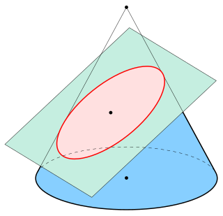
<span class="mw-page-title-main">Ellipse</span> Plane curve: conic section

In mathematics, an ellipse is a plane curve surrounding two focal points, such that for all points on the curve, the sum of the two distances to the focal points is a constant. It generalizes a circle, which is the special type of ellipse in which the two focal points are the same. The elongation of an ellipse is measured by its eccentricity $, a number ranging from to .$

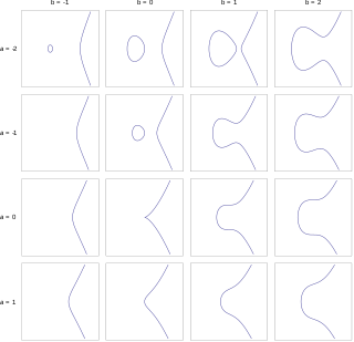
<span class="mw-page-title-main">Elliptic curve</span> Algebraic curve

In mathematics, an elliptic curve is a smooth, projective, algebraic curve of genus one, on which there is a specified point $O$ . An elliptic curve is defined over a field $K$ and describes points in $K 2$ , the Cartesian product of $K$ with itself. If the field's characteristic is different from 2 and 3, then the curve can be described as a plane algebraic curve which consists of solutions $(x, y)$ for:

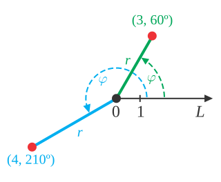
In mathematics, the polar coordinate system is a two-dimensional coordinate system in which each point on a plane is determined by a distance from a reference point and an angle from a reference direction. The reference point is called the pole, and the ray from the pole in the reference direction is the polar axis. The distance from the pole is called the radial coordinate, radial distance or simply radius, and the angle is called the angular coordinate, polar angle, or azimuth. Angles in polar notation are generally expressed in either degrees or radians.

In geometry, the tangent line (or simply tangent) to a plane curve at a given point is, intuitively, the straight line that "just touches" the curve at that point. Leibniz defined it as the line through a pair of infinitely close points on the curve. More precisely, a straight line is tangent to the curve y = f(x) at a point x = c if the line passes through the point (c, f(c)) on the curve and has slope f'(c), where f' is the derivative of f. A similar definition applies to space curves and curves in n-dimensional Euclidean space.

In mathematics and physics, Laplace's equation is a second-order partial differential equation named after Pierre-Simon Laplace, who first studied its properties. This is often written as $or where is the Laplace operator, is the divergence operator, is the gradient operator, and is a twice-differentiable real-valued function. The Laplace operator therefore maps a scalar function to another scalar function.$

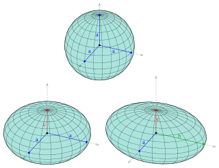
<span class="mw-page-title-main">Ellipsoid</span> Quadric surface that looks like a deformed sphere

An ellipsoid is a surface that can be obtained from a sphere by deforming it by means of directional scalings, or more generally, of an affine transformation.

The Lenstra elliptic-curve factorization or the elliptic-curve factorization method (ECM) is a fast, sub-exponential running time, algorithm for integer factorization, which employs elliptic curves. For general-purpose factoring, ECM is the third-fastest known factoring method. The second-fastest is the multiple polynomial quadratic sieve, and the fastest is the general number field sieve. The Lenstra elliptic-curve factorization is named after Hendrik Lenstra.

In mathematics, the Laplace operator or Laplacian is a differential operator given by the divergence of the gradient of a scalar function on Euclidean space. It is usually denoted by the symbols $, (where is the nabla operator), or . In a Cartesian coordinate system, the Laplacian is given by the sum of second partial derivatives of the function with respect to each independent variable. In other coordinate systems, such as cylindrical and spherical coordinates, the Laplacian also has a useful form. Informally, the Laplacian Δ f (p) of a function f at a point p measures by how much the average value of f over small spheres or balls centered at p deviates from f (p) .$

In mathematics, an affine algebraic plane curve is the zero set of a polynomial in two variables. A projective algebraic plane curve is the zero set in a projective plane of a homogeneous polynomial in three variables. An affine algebraic plane curve can be completed in a projective algebraic plane curve by homogenizing its defining polynomial. Conversely, a projective algebraic plane curve of homogeneous equation $h (x, y, t) = 0$ can be restricted to the affine algebraic plane curve of equation $h (x, y, 1) = 0$ . These two operations are each inverse to the other; therefore, the phrase algebraic plane curve is often used without specifying explicitly whether it is the affine or the projective case that is considered.

In differential geometry, the Ricci curvature tensor, named after Gregorio Ricci-Curbastro, is a geometric object which is determined by a choice of Riemannian or pseudo-Riemannian metric on a manifold. It can be considered, broadly, as a measure of the degree to which the geometry of a given metric tensor differs locally from that of ordinary Euclidean space or pseudo-Euclidean space.

In cryptography, the Elliptic Curve Digital Signature Algorithm (ECDSA) offers a variant of the Digital Signature Algorithm (DSA) which uses elliptic-curve cryptography.

In mathematics, a parametric equation defines a group of quantities as functions of one or more independent variables called parameters. Parametric equations are commonly used to express the coordinates of the points that make up a geometric object such as a curve or surface, called a parametric curve and parametric surface, respectively. In such cases, the equations are collectively called a parametric representation, or parametric system, or parameterization of the object.

<span class="mw-page-title-main">Dupin cyclide</span> Geometric inversion of a torus, cylinder or double cone

In mathematics, a Dupin cyclide or cyclide of Dupin is any geometric inversion of a standard torus, cylinder or double cone. In particular, these latter are themselves examples of Dupin cyclides. They were discovered c. 1802 by Charles Dupin, while he was still a student at the École polytechnique following Gaspard Monge's lectures. The key property of a Dupin cyclide is that it is a channel surface in two different ways. This property means that Dupin cyclides are natural objects in Lie sphere geometry.

In physics, the Hamilton–Jacobi equation, named after William Rowan Hamilton and Carl Gustav Jacob Jacobi, is an alternative formulation of classical mechanics, equivalent to other formulations such as Newton's laws of motion, Lagrangian mechanics and Hamiltonian mechanics.

In mathematics, the Helmholtz equation is the eigenvalue problem for the Laplace operator. It corresponds to the elliptic partial differential equation: $where \nabla 2 is the Laplace operator, k 2 is the eigenvalue, and f is the (eigen)function. When the equation is applied to waves, k is known as the wave number. The Helmholtz equation has a variety of applications in physics and other sciences, including the wave equation, the diffusion equation, and the Schrödinger equation for a free particle.$

In mathematics, the lemniscate elliptic functions are elliptic functions related to the arc length of the lemniscate of Bernoulli. They were first studied by Giulio Fagnano in 1718 and later by Leonhard Euler and Carl Friedrich Gauss, among others.

In geometry, the trilinear coordinates $x : y : z$ of a point relative to a given triangle describe the relative directed distances from the three sidelines of the triangle. Trilinear coordinates are an example of homogeneous coordinates. The ratio $x : y$ is the ratio of the perpendicular distances from the point to the sides opposite vertices $A$ and $B$ respectively; the ratio $y : z$ is the ratio of the perpendicular distances from the point to the sidelines opposite vertices $B$ and $C$ respectively; and likewise for $z : x$ and vertices $C$ and $A$ .

<span class="mw-page-title-main">Edwards curve</span>

In mathematics, the Edwards curves are a family of elliptic curves studied by Harold Edwards in 2007. The concept of elliptic curves over finite fields is widely used in elliptic curve cryptography. Applications of Edwards curves to cryptography were developed by Daniel J. Bernstein and Tanja Lange: they pointed out several advantages of the Edwards form in comparison to the more well known Weierstrass form.

In mathematics, the Twisted Hessian curve represents a generalization of Hessian curves; it was introduced in elliptic curve cryptography to speed up the addition and doubling formulas and to have strongly unified arithmetic. In some operations, it is close in speed to Edwards curves.

In Euclidean geometry, for a plane curve $C$ and a given fixed point $O$ , the pedal equation of the curve is a relation between $r$ and $p$ where $r$ is the distance from $O$ to a point on $C$ and $p$ is the perpendicular distance from $O$ to the tangent line to $C$ at the point. The point $O$ is called the pedal point and the values $r$ and $p$ are sometimes called the pedal coordinates of a point relative to the curve and the pedal point. It is also useful to measure the distance of $O$ to the normal $p c$ (the contrapedal coordinate) even though it is not an independent quantity and it relates to $(r, p)$ as

References

Peter L. Montgomery (1987). "Speeding the Pollard and Elliptic Curve Methods of Factorization". Mathematics of Computation. 48 (177): 243–264. doi: 10.2307/2007888 . JSTOR 2007888.
Daniel J. Bernstein, Peter Birkner, Marc Joye, Tanja Lange and Christiane Peters (2008). "Twisted Edwards Curves". Progress in Cryptology – AFRICACRYPT 2008. Lecture Notes in Computer Science. Vol. 5023. Springer-Verlag Berlin Heidelberg. pp. 389–405. doi:10.1007/978-3-540-68164-9_26. ISBN 978-3-540-68159-5.{{cite book}}: CS1 maint: multiple names: authors list (link)
Wouter Castryck; Steven Galbraith; Reza Rezaeian Farashahi (2008). "Efficient Arithmetic on Elliptic Curves using a Mixed Edwards-Montgomery Representation" (PDF).{{cite journal}}: Cite journal requires |journal= (help)

External links

Genus-1 curves over large-characteristic fields

This page is based on this Wikipedia article
Text is available under the CC BY-SA 4.0 license; additional terms may apply.
Images, videos and audio are available under their respective licenses.

[1] Peter L. Montgomery (1987). "Speeding the Pollard and Elliptic Curve Methods of Factorization". Mathematics of Computation. 48 (177): 243–264. doi: 10.2307/2007888 . JSTOR 2007888.

[2] Daniel J. Bernstein, Peter Birkner, Marc Joye, Tanja Lange and Christiane Peters (2008). "Twisted Edwards Curves". Progress in Cryptology – AFRICACRYPT 2008. Lecture Notes in Computer Science. Vol. 5023. Springer-Verlag Berlin Heidelberg. pp. 389–405. doi:10.1007/978-3-540-68164-9_26. ISBN 978-3-540-68159-5.{{cite book}}: CS1 maint: multiple names: authors list (link)

[3] Katsuyuki Okeya, Hiroyuki Kurumatani, and Kouichi Sakurai (2000). Elliptic Curves with the Montgomery-Form and Their Cryptographic Applications. Public Key Cryptography (PKC2000). doi: 10.1007/978-3-540-46588-1_17 .{{cite conference}}: CS1 maint: multiple names: authors list (link)

[1]

[2]

[3]