In machine learning, the perceptron is an algorithm for supervised learning of binary classifiers. A binary classifier is a function which can decide whether or not an input, represented by a vector of numbers, belongs to some specific class. It is a type of linear classifier, i.e. a classification algorithm that makes its predictions based on a linear predictor function combining a set of weights with the feature vector.
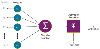
An artificial neuron is a mathematical function conceived as a model of biological neurons in a neural network. Artificial neurons are the elementary units of artificial neural networks. The artificial neuron is a function that receives one or more inputs, applies weights to these inputs, and sums them to produce an output.
Hebbian theory is a neuropsychological theory claiming that an increase in synaptic efficacy arises from a presynaptic cell's repeated and persistent stimulation of a postsynaptic cell. It is an attempt to explain synaptic plasticity, the adaptation of brain neurons during the learning process. It was introduced by Donald Hebb in his 1949 book The Organization of Behavior. The theory is also called Hebb's rule, Hebb's postulate, and cell assembly theory. Hebb states it as follows:
Let us assume that the persistence or repetition of a reverberatory activity tends to induce lasting cellular changes that add to its stability. ... When an axon of cell A is near enough to excite a cell B and repeatedly or persistently takes part in firing it, some growth process or metabolic change takes place in one or both cells such that A’s efficiency, as one of the cells firing B, is increased.
In signal processing, independent component analysis (ICA) is a computational method for separating a multivariate signal into additive subcomponents. This is done by assuming that at most one subcomponent is Gaussian and that the subcomponents are statistically independent from each other. ICA was invented by Jeanny Hérault and Christian Jutten in 1985. ICA is a special case of blind source separation. A common example application of ICA is the "cocktail party problem" of listening in on one person's speech in a noisy room.
A Hopfield network is a form of recurrent neural network, or a spin glass system, that can serve as a content-addressable memory. The Hopfield network, named for John Hopfield, consists of a single layer of neurons, where each neuron is connected to every other neuron except itself. These connections are bidirectional and symmetric, meaning the weight of the connection from neuron i to neuron j is the same as the weight from neuron j to neuron i. Patterns are associatively recalled by fixing certain inputs, and dynamically evolve the network to minimize an energy function, towards local energy minimum states that correspond to stored patterns. Patterns are associatively learned by a Hebbian learning algorithm.
In machine learning, backpropagation is a gradient estimation method commonly used for training neural networks to compute the network parameter updates.

A feedforward neural network (FNN) is one of the two broad types of artificial neural network, characterized by direction of the flow of information between its layers. Its flow is uni-directional, meaning that the information in the model flows in only one direction—forward—from the input nodes, through the hidden nodes and to the output nodes, without any cycles or loops. Modern feedforward networks are trained using backpropagation, and are colloquially referred to as "vanilla" neural networks.
A multilayer perceptron (MLP) is a name for a modern feedforward artificial neural network, consisting of fully connected neurons with a nonlinear activation function, organized in at least three layers, notable for being able to distinguish data that is not linearly separable.
In machine learning, kernel machines are a class of algorithms for pattern analysis, whose best known member is the support-vector machine (SVM). These methods involve using linear classifiers to solve nonlinear problems. The general task of pattern analysis is to find and study general types of relations in datasets. For many algorithms that solve these tasks, the data in raw representation have to be explicitly transformed into feature vector representations via a user-specified feature map: in contrast, kernel methods require only a user-specified kernel, i.e., a similarity function over all pairs of data points computed using inner products. The feature map in kernel machines is infinite dimensional but only requires a finite dimensional matrix from user-input according to the Representer theorem. Kernel machines are slow to compute for datasets larger than a couple of thousand examples without parallel processing.
The softmax function, also known as softargmax or normalized exponential function, converts a vector of K real numbers into a probability distribution of K possible outcomes. It is a generalization of the logistic function to multiple dimensions, and is used in multinomial logistic regression. The softmax function is often used as the last activation function of a neural network to normalize the output of a network to a probability distribution over predicted output classes.
ADALINE is an early single-layer artificial neural network and the name of the physical device that implemented this network. It was developed by professor Bernard Widrow and his doctoral student Ted Hoff at Stanford University in 1960. It is based on the perceptron. It consists of weights, a bias and a summation function. The weights and biases were implemented by rheostats, and later, memistors.
In the field of mathematical modeling, a radial basis function network is an artificial neural network that uses radial basis functions as activation functions. The output of the network is a linear combination of radial basis functions of the inputs and neuron parameters. Radial basis function networks have many uses, including function approximation, time series prediction, classification, and system control. They were first formulated in a 1988 paper by Broomhead and Lowe, both researchers at the Royal Signals and Radar Establishment.
Neural cryptography is a branch of cryptography dedicated to analyzing the application of stochastic algorithms, especially artificial neural network algorithms, for use in encryption and cryptanalysis.
BCM theory, BCM synaptic modification, or the BCM rule, named for Elie Bienenstock, Leon Cooper, and Paul Munro, is a physical theory of learning in the visual cortex developed in 1981. The BCM model proposes a sliding threshold for long-term potentiation (LTP) or long-term depression (LTD) induction, and states that synaptic plasticity is stabilized by a dynamic adaptation of the time-averaged postsynaptic activity. According to the BCM model, when a pre-synaptic neuron fires, the post-synaptic neurons will tend to undergo LTP if it is in a high-activity state, or LTD if it is in a lower-activity state. This theory is often used to explain how cortical neurons can undergo both LTP or LTD depending on different conditioning stimulus protocols applied to pre-synaptic neurons.
The generalized Hebbian algorithm (GHA), also known in the literature as Sanger's rule, is a linear feedforward neural network for unsupervised learning with applications primarily in principal components analysis. First defined in 1989, it is similar to Oja's rule in its formulation and stability, except it can be applied to networks with multiple outputs. The name originates because of the similarity between the algorithm and a hypothesis made by Donald Hebb about the way in which synaptic strengths in the brain are modified in response to experience, i.e., that changes are proportional to the correlation between the firing of pre- and post-synaptic neurons.
In neuroscience and computer science, synaptic weight refers to the strength or amplitude of a connection between two nodes, corresponding in biology to the amount of influence the firing of one neuron has on another. The term is typically used in artificial and biological neural network research.
Competitive learning is a form of unsupervised learning in artificial neural networks, in which nodes compete for the right to respond to a subset of the input data. A variant of Hebbian learning, competitive learning works by increasing the specialization of each node in the network. It is well suited to finding clusters within data.
In machine learning, particularly in the creation of artificial neural networks, ensemble averaging is the process of creating multiple models and combining them to produce a desired output, as opposed to creating just one model. Frequently an ensemble of models performs better than any individual model, because the various errors of the models "average out."
An artificial neural network's learning rule or learning process is a method, mathematical logic or algorithm which improves the network's performance and/or training time. Usually, this rule is applied repeatedly over the network. It is done by updating the weights and bias levels of a network when a network is simulated in a specific data environment. A learning rule may accept existing conditions of the network and will compare the expected result and actual result of the network to give new and improved values for weights and bias. Depending on the complexity of actual model being simulated, the learning rule of the network can be as simple as an XOR gate or mean squared error, or as complex as the result of a system of differential equations.
An artificial neural network (ANN) combines biological principles with advanced statistics to solve problems in domains such as pattern recognition and game-play. ANNs adopt the basic model of neuron analogues connected to each other in a variety of ways.


