In mathematics, an ellipse is a plane curve surrounding two focal points, such that for all points on the curve, the sum of the two distances to the focal points is a constant. It generalizes a circle, which is the special type of ellipse in which the two focal points are the same. The elongation of an ellipse is measured by its eccentricity , a number ranging from to .

In mathematics, a spherical coordinate system is a coordinate system for three-dimensional space where the position of a point is specified by three numbers: the radial distance of that point from a fixed origin; its polar angle measured from a fixed polar axis or zenith direction; and the azimuthal angle of its orthogonal projection on a reference plane that passes through the origin and is orthogonal to the fixed axis, measured from another fixed reference direction on that plane. When radius is fixed, the two angular coordinates make a coordinate system on the sphere sometimes called spherical polar coordinates.

In mathematics, an n-sphere or a hypersphere is a topological space that is homeomorphic to a standardn-sphere, which is the set of points in (n + 1)-dimensional Euclidean space that are situated at a constant distance r from a fixed point, called the center. It is the generalization of an ordinary sphere in the ordinary three-dimensional space. The "radius" of a sphere is the constant distance of its points to the center. When the sphere has unit radius, it is usual to call it the unit n-sphere or simply the n-sphere for brevity. In terms of the standard norm, the n-sphere is defined as
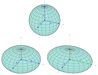
An ellipsoid is a surface that can be obtained from a sphere by deforming it by means of directional scalings, or more generally, of an affine transformation.
In mathematics, a Gaussian function, often simply referred to as a Gaussian, is a function of the base form

The Fresnel integralsS(x) and C(x) are two transcendental functions named after Augustin-Jean Fresnel that are used in optics and are closely related to the error function (erf). They arise in the description of near-field Fresnel diffraction phenomena and are defined through the following integral representations:

In mathematics, the inverse trigonometric functions are the inverse functions of the trigonometric functions. Specifically, they are the inverses of the sine, cosine, tangent, cotangent, secant, and cosecant functions, and are used to obtain an angle from any of the angle's trigonometric ratios. Inverse trigonometric functions are widely used in engineering, navigation, physics, and geometry.
In differential geometry, the first fundamental form is the inner product on the tangent space of a surface in three-dimensional Euclidean space which is induced canonically from the dot product of R3. It permits the calculation of curvature and metric properties of a surface such as length and area in a manner consistent with the ambient space. The first fundamental form is denoted by the Roman numeral I,

In mathematics, physics and engineering, the sinc function, denoted by sinc(x), has two forms, normalized and unnormalized.

In mathematics, a rose or rhodonea curve is a sinusoid specified by either the cosine or sine functions with no phase angle that is plotted in polar coordinates. Rose curves or "rhodonea" were named by the Italian mathematician who studied them, Guido Grandi, between the years 1723 and 1728.
This is a table of orthonormalized spherical harmonics that employ the Condon-Shortley phase up to degree . Some of these formulas are expressed in terms of the Cartesian expansion of the spherical harmonics into polynomials in x, y, z, and r. For purposes of this table, it is useful to express the usual spherical to Cartesian transformations that relate these Cartesian components to and as
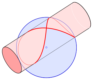
In mathematics, Viviani's curve, also known as Viviani's window, is a figure eight shaped space curve named after the Italian mathematician Vincenzo Viviani. It is the intersection of a sphere with a cylinder that is tangent to the sphere and passes through two poles of the sphere. Before Viviani this curve was studied by Simon de La Loubère and Gilles de Roberval.
In Hamiltonian mechanics, the linear canonical transformation (LCT) is a family of integral transforms that generalizes many classical transforms. It has 4 parameters and 1 constraint, so it is a 3-dimensional family, and can be visualized as the action of the special linear group SL2(R) on the time–frequency plane (domain). As this defines the original function up to a sign, this translates into an action of its double cover on the original function space.
In mathematics, sine and cosine are trigonometric functions of an angle. The sine and cosine of an acute angle are defined in the context of a right triangle: for the specified angle, its sine is the ratio of the length of the side that is opposite that angle to the length of the longest side of the triangle, and the cosine is the ratio of the length of the adjacent leg to that of the hypotenuse. For an angle , the sine and cosine functions are denoted simply as and .
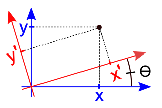
In mathematics, a rotation of axes in two dimensions is a mapping from an xy-Cartesian coordinate system to an x′y′-Cartesian coordinate system in which the origin is kept fixed and the x′ and y′ axes are obtained by rotating the x and y axes counterclockwise through an angle . A point P has coordinates (x, y) with respect to the original system and coordinates (x′, y′) with respect to the new system. In the new coordinate system, the point P will appear to have been rotated in the opposite direction, that is, clockwise through the angle . A rotation of axes in more than two dimensions is defined similarly. A rotation of axes is a linear map and a rigid transformation.
There are several equivalent ways for defining trigonometric functions, and the proof of the trigonometric identities between them depend on the chosen definition. The oldest and somehow the most elementary definition is based on the geometry of right triangles. The proofs given in this article use this definition, and thus apply to non-negative angles not greater than a right angle. For greater and negative angles, see Trigonometric functions.

In mathematics, the axis–angle representation of a rotation parameterizes a rotation in a three-dimensional Euclidean space by two quantities: a unit vector e indicating the direction of an axis of rotation, and an angle θ describing the magnitude of the rotation about the axis. Only two numbers, not three, are needed to define the direction of a unit vector e rooted at the origin because the magnitude of e is constrained. For example, the elevation and azimuth angles of e suffice to locate it in any particular Cartesian coordinate frame.
Common integrals in quantum field theory are all variations and generalizations of Gaussian integrals to the complex plane and to multiple dimensions. Other integrals can be approximated by versions of the Gaussian integral. Fourier integrals are also considered.
The direct-quadrature-zerotransformation or zero-direct-quadraturetransformation is a tensor that rotates the reference frame of a three-element vector or a three-by-three element matrix in an effort to simplify analysis. The DQZ transform is the product of the Clarke transform and the Park transform, first proposed in 1929 by Robert H. Park.