In computer science, a double-ended queue is an abstract data type that generalizes a queue, for which elements can be added to or removed from either the front (head) or back (tail). It is also often called a head-tail linked list, though properly this refers to a specific data structure implementation of a deque.

In computing, a hash table, also known as a hash map or a hash set, is a data structure that implements an associative array, also called a dictionary, which is an abstract data type that maps keys to values. A hash table uses a hash function to compute an index, also called a hash code, into an array of buckets or slots, from which the desired value can be found. During lookup, the key is hashed and the resulting hash indicates where the corresponding value is stored.
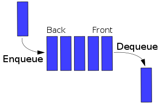
In computer science, a queue is a collection of entities that are maintained in a sequence and can be modified by the addition of entities at one end of the sequence and the removal of entities from the other end of the sequence. By convention, the end of the sequence at which elements are added is called the back, tail, or rear of the queue, and the end at which elements are removed is called the head or front of the queue, analogously to the words used when people line up to wait for goods or services.
A splay tree is a binary search tree with the additional property that recently accessed elements are quick to access again. Like self-balancing binary search trees, a splay tree performs basic operations such as insertion, look-up and removal in O(log n) amortized time. For random access patterns drawn from a non-uniform random distribution, their amortized time can be faster than logarithmic, proportional to the entropy of the access pattern. For many patterns of non-random operations, also, splay trees can take better than logarithmic time, without requiring advance knowledge of the pattern. According to the unproven dynamic optimality conjecture, their performance on all access patterns is within a constant factor of the best possible performance that could be achieved by any other self-adjusting binary search tree, even one selected to fit that pattern. The splay tree was invented by Daniel Sleator and Robert Tarjan in 1985.

An ideal gas is a theoretical gas composed of many randomly moving point particles that are not subject to interparticle interactions. The ideal gas concept is useful because it obeys the ideal gas law, a simplified equation of state, and is amenable to analysis under statistical mechanics. The requirement of zero interaction can often be relaxed if, for example, the interaction is perfectly elastic or regarded as point-like collisions.
In computer science, amortized analysis is a method for analyzing a given algorithm's complexity, or how much of a resource, especially time or memory, it takes to execute. The motivation for amortized analysis is that looking at the worst-case run time can be too pessimistic. Instead, amortized analysis averages the running times of operations in a sequence over that sequence. As a conclusion: "Amortized analysis is a useful tool that complements other techniques such as worst-case and average-case analysis."
In computer science, a Fibonacci heap is a data structure for priority queue operations. It has a better amortized running time than many other priority queue data structures including the binary heap and binomial heap. consisting of a collection of heap-ordered trees. Michael L. Fredman and Robert E. Tarjan developed Fibonacci heaps in 1984 and published them in a scientific journal in 1987. Fibonacci heaps are named after the Fibonacci numbers, which are used in their running time analysis.
In computing, a persistent data structure or not ephemeral data structure is a data structure that always preserves the previous version of itself when it is modified. Such data structures are effectively immutable, as their operations do not (visibly) update the structure in-place, but instead always yield a new updated structure. The term was introduced in Driscoll, Sarnak, Sleator, and Tarjan's 1986 article.
In computer science, a disjoint-set data structure, also called a union–find data structure or merge–find set, is a data structure that stores a collection of disjoint (non-overlapping) sets. Equivalently, it stores a partition of a set into disjoint subsets. It provides operations for adding new sets, merging sets, and finding a representative member of a set. The last operation makes it possible to find out efficiently if any two elements are in the same or different sets.

In system analysis, among other fields of study, a linear time-invariant (LTI) system is a system that produces an output signal from any input signal subject to the constraints of linearity and time-invariance; these terms are briefly defined below. These properties apply (exactly or approximately) to many important physical systems, in which case the response y(t) of the system to an arbitrary input x(t) can be found directly using convolution: y(t) = (x ∗ h)(t) where h(t) is called the system's impulse response and ∗ represents convolution (not to be confused with multiplication). What's more, there are systematic methods for solving any such system (determining h(t)), whereas systems not meeting both properties are generally more difficult (or impossible) to solve analytically. A good example of an LTI system is any electrical circuit consisting of resistors, capacitors, inductors and linear amplifiers.

In computer science, a dynamic array, growable array, resizable array, dynamic table, mutable array, or array list is a random access, variable-size list data structure that allows elements to be added or removed. It is supplied with standard libraries in many modern mainstream programming languages. Dynamic arrays overcome a limit of static arrays, which have a fixed capacity that needs to be specified at allocation.

In mathematics, a flow formalizes the idea of the motion of particles in a fluid. Flows are ubiquitous in science, including engineering and physics. The notion of flow is basic to the study of ordinary differential equations. Informally, a flow may be viewed as a continuous motion of points over time. More formally, a flow is a group action of the real numbers on a set.
In theoretical physics, a scalar–tensor theory is a field theory that includes both a scalar field and a tensor field to represent a certain interaction. For example, the Brans–Dicke theory of gravitation uses both a scalar field and a tensor field to mediate the gravitational interaction.
In theoretical physics, scalar field theory can refer to a relativistically invariant classical or quantum theory of scalar fields. A scalar field is invariant under any Lorentz transformation.

In computer science, a hashed array tree (HAT) is a dynamic array data-structure published by Edward Sitarski in 1996, maintaining an array of separate memory fragments to store the data elements, unlike simple dynamic arrays which maintain their data in one contiguous memory area. Its primary objective is to reduce the amount of element copying due to automatic array resizing operations, and to improve memory usage patterns.
In computer science, a finger tree is a purely functional data structure that can be used to efficiently implement other functional data structures. A finger tree gives amortized constant time access to the "fingers" (leaves) of the tree, which is where data is stored, and concatenation and splitting logarithmic time in the size of the smaller piece. It also stores in each internal node the result of applying some associative operation to its descendants. This "summary" data stored in the internal nodes can be used to provide the functionality of data structures other than trees.

In physics, a gauge theory is a type of field theory in which the Lagrangian, and hence the dynamics of the system itself, do not change under local transformations according to certain smooth families of operations. Formally, the Lagrangian is invariant.

In computer science, a queap is a priority queue data structure. The data structure allows insertions and deletions of arbitrary elements, as well as retrieval of the highest-priority element. Each deletion takes amortized time logarithmic in the number of items that have been in the structure for a longer time than the removed item. Insertions take constant amortized time.
The quantum cylindrical quadrupole is a solution to the Schrödinger equation, where is the reduced Planck constant, is the mass of the particle, is the imaginary unit and is time.
A monoque is a linear data structure which provides dynamic array semantics. A monoque is similar in structure to a deque but is limited to operations on one end. Hence the name, mono-que. A monoque offers O(1) random access and O(1) push_back/pop_back. Unlike a C++ vector, the push_back/pop_back functions are not amortized and are strictly O(1) in time complexity. Because the block list is never reallocated or resized, it maintains strictly O(1) non-amortized worst case performance. Unlike C++'s deque, the O(1) performance guarantee includes the time complexity of working with the block list, whereas the C++ standard only guarantees the deque to be O(1) in terms of operations on the underlying value type.


