Principles of grid generation

Last updated June 25, 2022

Grids or meshes are geometrical shapes (formed after discretisation of the geometric domain) which are small-sized discrete cells that cover the physical domain, whose objective is to identify the discrete volumes or elements where conservation laws can be applied. They have applications in the fields of computational fluid dynamics (CFD), geography, designing and many more places where numerical solutions to the partial differential equations (PDEs) are required.

Numerical grid generation is the crucial initial step involved in computing numerical solutions to the equations that describe a physical process. The accuracy of the solution depends upon the quality of the grid generated. A well-constructed grid can improve the quality of solution whereas, deviations from the numerical solution can be observed with a poorly constructed grid. Techniques for creating the cell forms the basis of grid generation. Various methods for the grid generation are discussed below.

Algebraic methods

The grid generation by algebraic methods is based on mathematical interpolation function. It is done by using known functions in one, two or three dimensions taking arbitrary shaped regions. The computational domain might not be rectangular, but for the sake of simplicity, the domain is taken to be rectangular. The main advantage of the methods is that they provide explicit control of physical grid shape and spacing. The simplest procedure that may be used to produce boundary fitted computational mesh is the normalization transformation.^[1]
For a nozzle, with the describing function $y=x^{2}$ the grid can easily be generated using uniform division in y-direction with equally spaced increments in x-direction, which are described by

\xi =x\,

\eta ={\frac {y}{y_{\max }}}\,

where $y_{\max }$ denotes the y-coordinate of the nozzle wall. For given values of ( $\xi$ , $\eta$ ), the values of ( $x$ , $y$ ) can be easily recovered.

Differential equation methods

Like algebraic methods, differential equation methods are also used to generate grids. The advantage of using the partial differential equations (PDEs) is that the solution of grid generating equations can be exploited to generate the mesh. Grid construction can be done using all three classes of partial differential equations.

Elliptic schemes

Elliptic PDEs generally have very smooth solutions leading to smooth contours. Using its smoothness as an advantage Laplace's equations can preferably be used because the Jacobian found out to be positive as a result of maximum principle for harmonic functions. After extensive work done by Crowley (1962) and Winslow (1966)^[2] on PDEs by transforming physical domain into computational plane while mapping using Poisson’s equation, Thompson et al. (1974)^[3] have worked extensively on elliptic PDEs to generate grids. In Poisson grid generators, the mapping is accomplished by marking the desired grid points $(x,y)$ on the boundary of the physical domain, with the interior point distribution determined through the solution of equations written below

\xi _{xx}+\xi _{yy}=P(\xi ,\eta )

\eta _{xx}+\eta _{yy}=Q(\xi ,\eta )

where, $(\xi ,\eta )$ are the co-ordinates in the computational domain, while P and Q are responsible for point spacing within D. Transforming above equations in computational space yields a set of two elliptic PDEs of the form,

\alpha x_{\xi \xi }-2\beta x_{\xi \eta }+\gamma x_{\eta \eta }=-I^{2}(Px_{\xi }+Qx_{\eta })

\alpha y_{\xi \xi }-2\beta y_{\xi \eta }+\gamma y_{\eta \eta }=-I^{2}(Py_{\xi }+Qy_{\eta })

where

{\begin{aligned}\alpha &=x_{\eta }^{2}+y_{\eta }^{2}\\\beta &=x_{\eta }x_{\xi }+y_{\xi }y_{\eta }\\\gamma &=x_{\xi }^{2}+y_{\xi }^{2}\\I&={\frac {\delta (x,y)}{\delta (\xi ,\eta )}}=y_{\eta }x_{\xi }-y_{\xi }x_{\eta }\end{aligned}}

These systems of equations are solved in the computational plane on uniformly spaced grid which provides us with the $(x,y)$ co-ordinates of each point in physical space. The advantage of using elliptic PDEs is the solution linked to them is smooth and the resulting grid is smooth. But, specification of P and Q becomes a difficult task thus adding it to its disadvantages. Moreover, the grid has to be computed after each time step which adds up to computational time.^[4]

Hyperbolic schemes

This grid generation scheme is generally applicable to problems with open domains consistent with the type of PDE describing the physical problem. The advantage associated with hyperbolic PDEs is that the governing equations need to be solved only once for generating grid. The initial point distribution along with the approximate boundary conditions forms the required input and the solution is the then marched outward. Steger and Sorenson (1980)^[5] proposed a volume orthogonality method that uses Hyperbolic PDEs for mesh generation. For a 2-D problem, Considering computational space to be given by $\Delta \xi =\Delta \eta =1$ , the inverse of the Jacobian is given by,

x_{\xi }y_{\eta }-x_{\eta }y_{\xi }=I

where $I$ represents the area in physical space for a given area in computational space. The second equation links the orthogonality of grid lines at the boundary in physical space which can be written as

d\xi =0=\xi _{x}\,dx+\xi _{y}\,dy.

For $\xi$ and $\eta$ surfaces to be perpendicular the equation becomes

x_{\xi }x_{\eta }+y_{\xi }y_{\eta }=0.

The problem associated with such system of equations is the specification of $I$ . Poor selection of $I$ may lead to shock and discontinuous propagation of this information throughout the mesh. While mesh being orthogonal is generated very rapidly which comes out as an advantage with this method.

Parabolic schemes

The solving technique is similar to that of hyperbolic PDEs by advancing the solution away from the initial data surface satisfying the boundary conditions at the end. Nakamura (1982) and Edwards (1985) developed the basic ideas for parabolic grid generation. The idea uses either of Laplace or the Poisson's equation and especially treating the parts which controls elliptic behavior. The initial values are given as the coordinates of the point along the surface $\eta =0$ and the advancing the solutions to the outer surface of the object satisfying the boundary conditions along $\xi$ edges.

The control of the grid spacing has not been suggested till now. Nakamura and Edwards, grid control was accomplished using non uniform spacing. The parabolic grid generation shows an advantage over the hyperbolic grid generation that, no shocks or discontinuities occur and the grid is relatively smooth. The specifications of initial values and selection of step size to control the grid points is however time consuming, but these techniques can be effective when familiarity and experience is gained.

Variational methods

This method includes a technique that minimizes grid smoothness, orthogonality and volume variation. This method forms mathematical platform to solve grid generation problems. In this method an alternative grid is generated by a new mesh after each iteration and computing the grid speed using backward difference method. This technique is a powerful one with a disadvantage that effort is required to solve the equations related to grid. Further work needed to be done to minimize the integrals that will reduce the CPU time.

Unstructured grid generation

See also Mesh generation. The main importance of this scheme is that it provides a method that will generate the grid automatically. Using this method, grids are segmented into blocks according to the surface of the element and a structure is provided to ensure appropriate connectivity. To interpret the data flow solver is used. When an unstructured scheme is employed, the main interest is to fulfill the demand of the user and a grid generator is used to accomplish this task. The information storage in structured scheme is cell to cell instead of grid to grid and hence the more memory space is needed. Due to random cell location, the solver efficiency in unstructured is less as compared to the structured scheme.^[6]

Some points are needed to be kept in mind at the time of grid construction. The grid point with high resolution creates difficulty for both structured and unstructured. For example, in case of boundary layer, structured scheme produces elongated grid in the direction of flow. On the other hand unstructured grids require a higher cell density in the boundary layer because the cell needs to be as equilateral as possible to avoid errors.^[7]

Connectivity information

We must identify what information is required to identify the cell and all the neighbors of the cell in the computational mesh. We can choose to locate the arbitrary points anywhere we want for the unstructured grid. A point insertion scheme is used to insert the points independently and the cell connectivity is determined. This suggests that the point be identified as they are inserted. Logic for establishing new connectivity is determined once the points are inserted. Data that form grid point that identifies grid cell are needed. As each cell is formed it is numbered and the points are sorted. In addition the neighbor cell information is needed.

Adaptive grid

A problem in solving partial differential equations using previous methods is that the grid is constructed and the points are distributed in the physical domain before details of the solution is known. So the grid may or may not be the best for the given problem.^[8]

Adaptive methods are used to improve the accuracy of the solutions. The adaptive method is referred to as ‘h’ method if mesh refinement is used, ‘r’ method if the number of grid point is fixed and not redistributed and ‘p’ if the order of solution scheme is increased in finite-element theory. The multi dimensional problems using the equidistribution scheme can be accomplished in several ways. The simplest to understand are the Poisson Grid Generators with control function based on the equidistribution of the weight function with the diffusion set as a multiple of desired cell volume. The equidistribution scheme can also be applied to the unstructured problem. The problem is the connectivity hampers if mesh point movement is very large.

Steady flow and the time-accurate flow calculation can be solved through this adaptive method. The grid is refined and after a predetermined number of iteration in order to adapt it in a steady flow problem. The grid will stop adjusting to the changes once the solution converges. In time accurate case coupling of the partial differential equations of the physical problem and those describing the grid movement is required.

Related Research Articles

In mathematics, a partial differential equation (PDE) is an equation which imposes relations between the various partial derivatives of a multivariable function.

The finite volume method (FVM) is a method for representing and evaluating partial differential equations in the form of algebraic equations. In the finite volume method, volume integrals in a partial differential equation that contain a divergence term are converted to surface integrals, using the divergence theorem. These terms are then evaluated as fluxes at the surfaces of each finite volume. Because the flux entering a given volume is identical to that leaving the adjacent volume, these methods are conservative. Another advantage of the finite volume method is that it is easily formulated to allow for unstructured meshes. The method is used in many computational fluid dynamics packages. "Finite volume" refers to the small volume surrounding each node point on a mesh.

Second-order linear partial differential equations (PDEs) are classified as either elliptic, hyperbolic, or parabolic. Any second-order linear PDE in two variables can be written in the form

Numerical methods for partial differential equations is the branch of numerical analysis that studies the numerical solution of partial differential equations (PDEs).

Computational electromagnetics Branch of physics

Computational electromagnetics (CEM), computational electrodynamics or electromagnetic modeling is the process of modeling the interaction of electromagnetic fields with physical objects and the environment.

In physics and fluid mechanics, a Blasius boundary layer describes the steady two-dimensional laminar boundary layer that forms on a semi-infinite plate which is held parallel to a constant unidirectional flow. Falkner and Skan later generalized Blasius' solution to wedge flow, i.e. flows in which the plate is not parallel to the flow.

In mathematics, and specifically partial differential equations (PDEs), d'Alembert's formula is the general solution to the one-dimensional wave equation $.$

An eikonal equation is a non-linear first-order partial differential equation that is encountered in problems of wave propagation.

In numerical analysis, finite-difference methods (FDM) are a class of numerical techniques for solving differential equations by approximating derivatives with finite differences. Both the spatial domain and time interval are discretized, or broken into a finite number of steps, and the value of the solution at these discrete points is approximated by solving algebraic equations containing finite differences and values from nearby points.

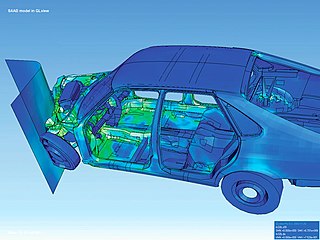
The finite element method (FEM) is a popular method for numerically solving differential equations arising in engineering and mathematical modeling. Typical problem areas of interest include the traditional fields of structural analysis, heat transfer, fluid flow, mass transport, and electromagnetic potential.

Miniaturizing components has always been a primary goal in the semiconductor industry because it cuts production cost and lets companies build smaller computers and other devices. Miniaturization, however, has increased dissipated power per unit area and made it a key limiting factor in integrated circuit performance. Temperature increase becomes relevant for relatively small-cross-sections wires, where it may affect normal semiconductor behavior. Besides, since the generation of heat is proportional to the frequency of operation for switching circuits, fast computers have larger heat generation than slow ones, an undesired effect for chips manufacturers. This article summaries physical concepts that describe the generation and conduction of heat in an integrated circuit, and presents numerical methods that model heat transfer from a macroscopic point of view.

Isogeometric analysis is a computational approach that offers the possibility of integrating finite element analysis (FEA) into conventional NURBS-based CAD design tools. Currently, it is necessary to convert data between CAD and FEA packages to analyse new designs during development, a difficult task since the two computational geometric approaches are different. Isogeometric analysis employs complex NURBS geometry in the FEA application directly. This allows models to be designed, tested and adjusted in one go, using a common data set.

In numerical mathematics, the boundary knot method (BKM) is proposed as an alternative boundary-type meshfree distance function collocation scheme.

The Kansa method is a computer method used to solve partial differential equations. Its main advantage is it is very easy to understand and program on a computer. It is much less complicated than the finite element method. Another advantage is it works well on multi variable problems. The finite element method is complicated when working with more than 3 space variables and time.

A mesh is a representation of a larger geometric domain by smaller discrete cells. Meshes are commonly used to compute solutions of partial differential equations and render computer graphics, and to analyze geographical and cartographic data. A mesh partitions space into elements over which the equations can be solved, which then approximates the solution over the larger domain. Element boundaries may be constrained to lie on internal or external boundaries within a model. Higher-quality (better-shaped) elements have better numerical properties, where what constitutes a "better" element depends on the general governing equations and the particular solution to the model instance.

Grid or mesh is defined as smaller shapes formed after discretisation of geometric domain. Mesh or grid can be in 3- dimension and 2-dimension. Meshing has applications in the fields of geography, designing, computational fluid dynamics. and many more places. The two-dimensional meshing includes simple polygon, polygon with holes, multiple domain and curved domain. In three dimensions there are three types of inputs. They are simple polyhedron, geometrical polyhedron and multiple polyhedrons. Before defining the mesh type it is necessary to understand elements.

In applied mathematics, oblate spheroidal wave functions are involved in the solution of the Helmholtz equation in oblate spheroidal coordinates. When solving this equation, $, by the method of separation of variables,, with:$

Fluid motion is governed by the Navier–Stokes equations, a set of coupled and nonlinear partial differential equations derived from the basic laws of conservation of mass, momentum and energy. The unknowns are usually the flow velocity, the pressure and density and temperature. The analytical solution of this equation is impossible hence scientists resort to laboratory experiments in such situations. The answers delivered are, however, usually qualitatively different since dynamical and geometric similitude are difficult to enforce simultaneously between the lab experiment and the prototype. Furthermore, the design and construction of these experiments can be difficult, particularly for stratified rotating flows. Computational fluid dynamics (CFD) is an additional tool in the arsenal of scientists. In its early days CFD was often controversial, as it involved additional approximation to the governing equations and raised additional (legitimate) issues. Nowadays CFD is an established discipline alongside theoretical and experimental methods. This position is in large part due to the exponential growth of computer power which has allowed us to tackle ever larger and more complex problems.

Mean-field particle methods are a broad class of interacting type Monte Carlo algorithms for simulating from a sequence of probability distributions satisfying a nonlinear evolution equation. These flows of probability measures can always be interpreted as the distributions of the random states of a Markov process whose transition probabilities depends on the distributions of the current random states. A natural way to simulate these sophisticated nonlinear Markov processes is to sample a large number of copies of the process, replacing in the evolution equation the unknown distributions of the random states by the sampled empirical measures. In contrast with traditional Monte Carlo and Markov chain Monte Carlo methods these mean-field particle techniques rely on sequential interacting samples. The terminology mean-field reflects the fact that each of the samples interacts with the empirical measures of the process. When the size of the system tends to infinity, these random empirical measures converge to the deterministic distribution of the random states of the nonlinear Markov chain, so that the statistical interaction between particles vanishes. In other words, starting with a chaotic configuration based on independent copies of initial state of the nonlinear Markov chain model, the chaos propagates at any time horizon as the size the system tends to infinity; that is, finite blocks of particles reduces to independent copies of the nonlinear Markov process. This result is called the propagation of chaos property. The terminology "propagation of chaos" originated with the work of Mark Kac in 1976 on a colliding mean-field kinetic gas model.

References

↑ Anderson, Dale (2012). Computational Fluid Mechanics and Heat Transfer, Third Edition Series in Computational and Physical Processes in Mechanics and Thermal Sciences. CRC Press. pp. 679–712. ISBN 978-1591690375.
↑ Winslow, A (1966). "Numerical Solution of Quasi-linear Poisson Equation". J. Comput. Phys. 1 (2): 149–172. doi:10.1016/0021-9991(66)90001-5.
↑ Thompson, J.F.; Thames, F.C.; Mastin, C.W. (1974). "Automatic Numerical Generation of Body-fitted Curvilinear Coordinate System for Field Containing any Number of Arbitrary Two-Dimensional Bodies". J. Comput. Phys. 15 (3): 299–319. doi:10.1016/0021-9991(74)90114-4.
↑ Young, David (1954). "Iterative methods for solving partial difference equations of elliptic type". Transactions of the American Mathematical Society. 76 (1): 92–111. doi: 10.2307/1990745 . ISSN 1088-6850. JSTOR 1990745.
↑ Steger, J.L; Sorenson, R.L (1980). "Use of hyperbolic partial differential equation to generate body fitted coordinates, Numerical Grid Generation Techniques" (PDF). NASA Conference Publication 2166: 463–478.
↑ Venkatakrishnan, V; Mavriplis, D. J (May 1991). "Implicit solvers for unstructured meshes". Journal of Computational Physics. 105 (1): 23. doi:10.1006/jcph.1993.1055. hdl: 2060/19910014812 .
↑ Weatherill, N.P (September 1992). "Delaunay triangulation in computational fluid dynamics". Computers & Mathematics with Applications. 24 (5–6): 129–150. doi: 10.1016/0898-1221(92)90045-j .
↑ Anderson, D.A; Sharpe H.N. (July 1993). "Orthogonal Adaptive Grid Generation with Fixed Internal Boundaries for Oil Reservoir Simulation". SPE Advanced Technology Series. 2. 1 (2): 53–62. doi:10.2118/21235-PA.

This page is based on this Wikipedia article
Text is available under the CC BY-SA 4.0 license; additional terms may apply.
Images, videos and audio are available under their respective licenses.

[1] Anderson, Dale (2012). Computational Fluid Mechanics and Heat Transfer, Third Edition Series in Computational and Physical Processes in Mechanics and Thermal Sciences. CRC Press. pp. 679–712. ISBN 978-1591690375.

[2] Winslow, A (1966). "Numerical Solution of Quasi-linear Poisson Equation". J. Comput. Phys. 1 (2): 149–172. doi:10.1016/0021-9991(66)90001-5.

[3] Thompson, J.F.; Thames, F.C.; Mastin, C.W. (1974). "Automatic Numerical Generation of Body-fitted Curvilinear Coordinate System for Field Containing any Number of Arbitrary Two-Dimensional Bodies". J. Comput. Phys. 15 (3): 299–319. doi:10.1016/0021-9991(74)90114-4.

[4] Young, David (1954). "Iterative methods for solving partial difference equations of elliptic type". Transactions of the American Mathematical Society. 76 (1): 92–111. doi: 10.2307/1990745 . ISSN 1088-6850. JSTOR 1990745.

[5] Steger, J.L; Sorenson, R.L (1980). "Use of hyperbolic partial differential equation to generate body fitted coordinates, Numerical Grid Generation Techniques" (PDF). NASA Conference Publication 2166: 463–478.

[6] Venkatakrishnan, V; Mavriplis, D. J (May 1991). "Implicit solvers for unstructured meshes". Journal of Computational Physics. 105 (1): 23. doi:10.1006/jcph.1993.1055. hdl: 2060/19910014812 .

[7] Weatherill, N.P (September 1992). "Delaunay triangulation in computational fluid dynamics". Computers & Mathematics with Applications. 24 (5–6): 129–150. doi: 10.1016/0898-1221(92)90045-j .

[8] Anderson, D.A; Sharpe H.N. (July 1993). "Orthogonal Adaptive Grid Generation with Fixed Internal Boundaries for Oil Reservoir Simulation". SPE Advanced Technology Series. 2. 1 (2): 53–62. doi:10.2118/21235-PA.

[1]

[2]

[3]

[4]

[5]

[6]

[7]

[8]