Solow residual

Last updated

The Solow residual is a number describing empirical productivity growth in an economy from year to year and decade to decade. Robert Solow, the Nobel Memorial Prize in Economic Sciences-winning economist, defined rising productivity as rising output with constant capital and labor input. It is a "residual" because it is the part of growth that is not accounted for by measures of capital accumulation or increased labor input. Increased physical throughput – i.e. environmental resources – is specifically excluded from the calculation; thus some portion of the residual can be ascribed to increased physical throughput. The example used is for the intracapital substitution of aluminium fixtures for steel during which the inputs do not alter. This differs in almost every other economic circumstance in which there are many other variables. The Solow residual is procyclical and measures of it are now called the rate of growth of multifactor productivity or total factor productivity, though Solow (1957) did not use these terms.

Contents

History

In the 1950s, many economists[ citation needed ] undertook comparative studies of economic growth following World War II reconstruction. Some[ who? ] said that the path to long-term growth was achieved through investment in industry and infrastructure and in moving further and further into capital intensive automated production. Although there was always a concern about diminishing returns to this approach because of equipment depreciation, it was a widespread view of the correct industrial policy to adopt. Many economists pointed to the Soviet command economy as a model of high-growth through tireless re-investment of output in further industrial construction.

However, some economists[ who? ] took a different view: they said that greater capital concentrations would yield diminishing returns once the marginal return to capital had equalized with that of labour – and that the apparently rapid growth of economies with high savings rates would be a short-term phenomenon. This analysis suggested[ citation needed ] that improved labour productivity or total factor technology was the long-run determinant of national growth, and that only under-capitalized countries could grow per-capita income substantially by investing in infrastructure – some of these undercapitalized countries were still recovering from the war and were expected to rapidly develop in this way on a path of convergence with developed nations.

The Solow residual is defined as per-capita economic growth above the rate of per-capita capital stock growth, so its detection indicates that there must be some contribution to output other than advances in industrializing the economy. The fact that the measured growth in the standard of living, also known as the ratio of output to labour input, could not be explained entirely by the growth in the capital/labour ratio was a significant finding, and pointed to innovation rather than capital accumulation as a potential path to growth.

The 'Solow growth model' is not intended to explain or derive the empirical residual, but rather to demonstrate how it will affect the economy in the long run when imposed on an aggregate model of the macroeconomy exogenously. This model was really a tool for demonstrating the impact of "technology" growth as against "industrial" growth rather than an attempt to understand where either type of growth was coming from. The Solow residual is primarily an observation to explain, rather than predict the outcome of a theoretical analysis. It is a question rather than an answer, and the following equations should not obscure that fact.

As a residual term in the Solow model

Solow assumed a very basic model of annual aggregate output over a year (t). He said that the output quantity would be governed by the amount of capital (the infrastructure), the amount of labour (the number of people in the workforce), and the productivity of that labour. He thought that the productivity of labour was the factor driving long-run GDP increases. An example economic model of this form is given below: [1]

where:

To measure or predict the change in output within this model, the equation above is differentiated in time (t), giving a formula in partial derivatives of the relationships: labour-to-output, capital-to-output, and productivity-to-output, as shown:

Observe:

Similarly:

and

Therefore:

The growth factor in the economy is a proportion of the output last year, which is given (assuming small changes year-on-year) by dividing both sides of this equation by the output, Y:

The first two terms on the right hand side of this equation are the proportional changes in labour and capital year-on-year, and the left hand side is the proportional output change. The remaining term on the right, giving the effect of productivity improvements on GDP is defined as the Solow residual:

The residual, SR(t) is that part of growth not explicable by measurable changes in the amount of capital, K, and the number of workers, L. If output, capital, and labour all double every twenty years the residual will be zero, but in general it is higher than this: output goes up faster than growth in the input factors. The residual varies between periods and countries, but is almost always positive in peace-time capitalist countries. Some estimates of the post-war U.S. residual credited the country with a 3% productivity increase per-annum until the early 1970s when productivity growth appeared to stagnate.

Regression analysis and the Solow residual

The above relation gives a very simplified picture of the economy in a single year; what growth theory econometrics does is to look at a sequence of years to find a statistically significant pattern in the changes of the variables, and perhaps identify the existence and value of the "Solow residual". The most basic technique for doing this is to assume constant rates of change in all the variables (obscured by noise), and regress on the data to find the best estimate of these rates in the historical data available (using an Ordinary least squares regression). Economists always do this by first taking the natural log of their equation (to separate out the variables on the right-hand-side of the equation); logging both sides of this production function produces a simple linear regression with an error term, :

A constant growth factor implies exponential growth in the above variables, so differentiating gives a linear relationship between the growth factors which can be deduced in a simple regression.

In a regression analysis, the equation one would estimate is:

where:

y is (log) output, ln(Y)

k is capital, ln(K)

is labour, ln(L)

C can be interpreted as the co-efficient on log(A) – the rate of technological change – (1  α).

Given the form of the regression equation, we can interpret the coefficients as elasticities.

For calculation of the actual quantity/ level of technology we simply refer back to our equation in levels.

Knowing quantities of output , capital , labor and estimates for , and we can solve for as:

Mankiw, Romer, and Weil augmented the Solow-Swan model with a human capital term. The explicit inclusion of this term in the model transfers the effect of changes in human capital from the Solow residual to capital accumulation. As a consequence, the Solow residual is smaller in the augmented Solow model:

where:

The associated regression to estimate this model is:

Breton estimates the Solow residual for the human capital-augmented version of the Solow-Swan model over the 20th century. [2] He finds that from 1910 to 2000 in 42 of the world's leading economies increased at an average rate of 1%/year and increased at 0.3%/year.

Why the productivity growth is attached to labor

The Solow residual measures total factor productivity, but the productivity variable is normally attached to the labor variable in the Solow-Swan model to make technological growth labor-augmenting. This type of productivity growth is required mathematically to keep the shares of national income accruing to the factors of production constant over time. These shares appear to have been stable historically in developing nations, and developed nations. [3] However, Thomas Piketty's famous study of inequality in 2014, using a version of the Solow model, argued that a stable, relatively low profit share of national income was largely a twentieth century phenomenon. [4]

Critique of the measurement in rapidly developing economies

Rapidly expanding countries (catching up after a crisis or trade liberalization) tend to have a rapid turn-over in technologies as they accumulate capital. It has been suggested that this will tend to make it harder to gain experience with the available technologies and that a zero Solow residual in these cases actually indicates rising labour productivity. In this theory, the fact that A (labour output productivity) is not falling as new skills become essential indicates that the labour force is capable of adapting, and is likely to have its productivity growth underestimated by the residual—This idea is linked to "learning-by-doing".

See also

Related Research Articles

<span class="mw-page-title-main">Exponential distribution</span> Probability distribution

In probability theory and statistics, the exponential distribution or negative exponential distribution is the probability distribution of the time between events in a Poisson point process, i.e., a process in which events occur continuously and independently at a constant average rate. It is a particular case of the gamma distribution. It is the continuous analogue of the geometric distribution, and it has the key property of being memoryless. In addition to being used for the analysis of Poisson point processes it is found in various other contexts.

Growth accounting is a procedure used in economics to measure the contribution of different factors to economic growth and to indirectly compute the rate of technological progress, measured as a residual, in an economy. Growth accounting decomposes the growth rate of an economy's total output into that which is due to increases in the contributing amount of the factors used—usually the increase in the amount of capital and labor—and that which cannot be accounted for by observable changes in factor utilization. The unexplained part of growth in GDP is then taken to represent increases in productivity or a measure of broadly defined technological progress.

<span class="mw-page-title-main">Least squares</span> Approximation method in statistics

The method of least squares is a standard approach in regression analysis to approximate the solution of overdetermined systems by minimizing the sum of the squares of the residuals made in the results of each individual equation.

<span class="mw-page-title-main">Beta distribution</span> Probability distribution

In probability theory and statistics, the beta distribution is a family of continuous probability distributions defined on the interval [0, 1] or in terms of two positive parameters, denoted by alpha (α) and beta (β), that appear as exponents of the variable and its complement to 1, respectively, and control the shape of the distribution.
<span class="mw-page-title-main">Logistic regression</span> Statistical model for a binary dependent variable

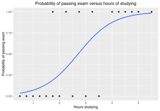
In statistics, the logistic model is a statistical model that models the probability of an event taking place by having the log-odds for the event be a linear combination of one or more independent variables. In regression analysis, logistic regression is estimating the parameters of a logistic model. Formally, in binary logistic regression there is a single binary dependent variable, coded by an indicator variable, where the two values are labeled "0" and "1", while the independent variables can each be a binary variable or a continuous variable. The corresponding probability of the value labeled "1" can vary between 0 and 1, hence the labeling; the function that converts log-odds to probability is the logistic function, hence the name. The unit of measurement for the log-odds scale is called a logit, from logistic unit, hence the alternative names. See § Background and § Definition for formal mathematics, and § Example for a worked example.

<span class="mw-page-title-main">Cobb–Douglas production function</span> Macroeconomic formula that describes productivity

In economics and econometrics, the Cobb–Douglas production function is a particular functional form of the production function, widely used to represent the technological relationship between the amounts of two or more inputs and the amount of output that can be produced by those inputs. The Cobb–Douglas form is developed and tested against statistical evidence by Charles Cobb and Paul Douglas between 1927 and 1947; according to Douglas, the functional form itself was developed earlier by Philip Wicksteed.

The Lotka–Volterra equations, also known as the Lotka–Volterra predator–prey model, are a pair of first-order nonlinear differential equations, frequently used to describe the dynamics of biological systems in which two species interact, one as a predator and the other as prey. The populations change through time according to the pair of equations:

<span class="mw-page-title-main">Nonlinear regression</span> Regression analysis

In statistics, nonlinear regression is a form of regression analysis in which observational data are modeled by a function which is a nonlinear combination of the model parameters and depends on one or more independent variables. The data are fitted by a method of successive approximations.

<span class="mw-page-title-main">Coefficient of determination</span> Indicator for how well data points fit a line or curve

In statistics, the coefficient of determination, denoted R2 or r2 and pronounced "R squared", is the proportion of the variation in the dependent variable that is predictable from the independent variable(s).

In statistics, ordinary least squares (OLS) is a type of linear least squares method for choosing the unknown parameters in a linear regression model by the principle of least squares: minimizing the sum of the squares of the differences between the observed dependent variable in the input dataset and the output of the (linear) function of the independent variable.

In economics, total-factor productivity (TFP), also called multi-factor productivity, is usually measured as the ratio of aggregate output to aggregate inputs. Under some simplifying assumptions about the production technology, growth in TFP becomes the portion of growth in output not explained by growth in traditionally measured inputs of labour and capital used in production. TFP is calculated by dividing output by the weighted geometric average of labour and capital input, with the standard weighting of 0.7 for labour and 0.3 for capital. Total factor productivity is a measure of productive efficiency in that it measures how much output can be produced from a certain amount of inputs. It accounts for part of the differences in cross-country per-capita income. For relatively small percentage changes, the rate of TFP growth can be estimated by subtracting growth rates of labor and capital inputs from the growth rate of output.

<span class="mw-page-title-main">Solow–Swan model</span> Model of long-run economic growth

The Solow–Swan model or exogenous growth model is an economic model of long-run economic growth. It attempts to explain long-run economic growth by looking at capital accumulation, labor or population growth, and increases in productivity largely driven by technological progress. At its core, it is an aggregate production function, often specified to be of Cobb–Douglas type, which enables the model "to make contact with microeconomics". The model was developed independently by Robert Solow and Trevor Swan in 1956, and superseded the Keynesian Harrod–Domar model.

<span class="mw-page-title-main">Simple linear regression</span> Linear regression model with a single explanatory variable

In statistics, simple linear regression is a linear regression model with a single explanatory variable. That is, it concerns two-dimensional sample points with one independent variable and one dependent variable and finds a linear function that, as accurately as possible, predicts the dependent variable values as a function of the independent variable. The adjective simple refers to the fact that the outcome variable is related to a single predictor.

<span class="mw-page-title-main">Ramsey–Cass–Koopmans model</span> Neoclassical economic model

The Ramsey–Cass–Koopmans model, or Ramsey growth model, is a neoclassical model of economic growth based primarily on the work of Frank P. Ramsey, with significant extensions by David Cass and Tjalling Koopmans. The Ramsey–Cass–Koopmans model differs from the Solow–Swan model in that the choice of consumption is explicitly microfounded at a point in time and so endogenizes the savings rate. As a result, unlike in the Solow–Swan model, the saving rate may not be constant along the transition to the long run steady state. Another implication of the model is that the outcome is Pareto optimal or Pareto efficient.

Non-linear least squares is the form of least squares analysis used to fit a set of m observations with a model that is non-linear in n unknown parameters (m ≥ n). It is used in some forms of nonlinear regression. The basis of the method is to approximate the model by a linear one and to refine the parameters by successive iterations. There are many similarities to linear least squares, but also some significant differences. In economic theory, the non-linear least squares method is applied in (i) the probit regression, (ii) threshold regression, (iii) smooth regression, (iv) logistic link regression, (v) Box–Cox transformed regressors ().

The Goodwin model, sometimes called Goodwin's class struggle model, is a model of endogenous economic fluctuations first proposed by the American economist Richard M. Goodwin in 1967. It combines aspects of the Harrod–Domar growth model with the Phillips curve to generate endogenous cycles in economic activity unlike most modern macroeconomic models in which movements in economic aggregates are driven by exogenously assumed shocks. Since Goodwin's publication in 1967, the model has been extended and applied in various ways.

In the technological theory of social production, the growth of output, measured in money units, is related to achievements in technological consumption of labour and energy. This theory is based on concepts of classical political economy and neo-classical economics and appears to be a generalisation of the known economic models, such as the neo-classical model of economic growth and input-output model.

Uzawa's theorem, also known as the steady state growth theorem, is a theorem in economic growth theory concerning the form that technological change can take in the Solow–Swan and Ramsey–Cass–Koopmans growth models. It was first proved by Japanese economist Hirofumi Uzawa.

<span class="mw-page-title-main">Hyperbolastic functions</span> Mathematical functions

The hyperbolastic functions, also known as hyperbolastic growth models, are mathematical functions that are used in medical statistical modeling. These models were originally developed to capture the growth dynamics of multicellular tumor spheres, and were introduced in 2005 by Mohammad Tabatabai, David Williams, and Zoran Bursac. The precision of hyperbolastic functions in modeling real world problems is somewhat due to their flexibility in their point of inflection. These functions can be used in a wide variety of modeling problems such as tumor growth, stem cell proliferation, pharma kinetics, cancer growth, sigmoid activation function in neural networks, and epidemiological disease progression or regression.

References

  1. This equation is a "Cobb–Douglas function", which is used more often than any other output relationship because of its analytical tractability, and because in the long-run, the precise relationship of capital to labour in the production function is not important. The same results can be derived with greater hardship using any production function having constant returns to scale (and satisfying the technical Inada conditions.)
  2. Breton, Theodore (2013). "World Productivity Growth and the Steady State Rate in the 20th Century". Economics Letters . 119 (3): 340–342. doi:10.1016/j.econlet.2013.03.013. hdl: 10784/2596 .
  3. Barro, Robert J.; Sala-i-Martin, Xavier (2004). "Growth Models with Exogenous Saving Rates". Economic Growth (Second ed.). New York: McGraw-Hill. pp. 23–84. ISBN   0-262-02553-1.
  4. Piketty, Thomas (2014). Capital in the Twenty-First Century . London: Harvard University Press. ISBN   9780674430006.

Further reading