
In mathematics and physics, Laplace's equation is a second-order partial differential equation named after Pierre-Simon Laplace, who first studied its properties. This is often written as

In physics, the Navier–Stokes equations are partial differential equations which describe the motion of viscous fluid substances, named after French engineer and physicist Claude-Louis Navier and Anglo-Irish physicist and mathematician George Gabriel Stokes. They were developed over several decades of progressively building the theories, from 1822 (Navier) to 1842-1850 (Stokes).
Linear elasticity is a mathematical model of how solid objects deform and become internally stressed due to prescribed loading conditions. It is a simplification of the more general nonlinear theory of elasticity and a branch of continuum mechanics.
In the calculus of variations, a field of mathematical analysis, the functional derivative relates a change in a functional to a change in a function on which the functional depends.

In fluid dynamics, the Euler equations are a set of quasilinear partial differential equations governing adiabatic and inviscid flow. They are named after Leonhard Euler. In particular, they correspond to the Navier–Stokes equations with zero viscosity and zero thermal conductivity.
In physics, the Hamilton–Jacobi equation, named after William Rowan Hamilton and Carl Gustav Jacob Jacobi, is an alternative formulation of classical mechanics, equivalent to other formulations such as Newton's laws of motion, Lagrangian mechanics and Hamiltonian mechanics. The Hamilton–Jacobi equation is particularly useful in identifying conserved quantities for mechanical systems, which may be possible even when the mechanical problem itself cannot be solved completely.
In the study of partial differential equations, the MUSCL scheme is a finite volume method that can provide highly accurate numerical solutions for a given system, even in cases where the solutions exhibit shocks, discontinuities, or large gradients. MUSCL stands for Monotonic Upstream-centered Scheme for Conservation Laws, and the term was introduced in a seminal paper by Bram van Leer. In this paper he constructed the first high-order, total variation diminishing (TVD) scheme where he obtained second order spatial accuracy.
In physics, the Green's function for Laplace's equation in three variables is used to describe the response of a particular type of physical system to a point source. In particular, this Green's function arises in systems that can be described by Poisson's equation, a partial differential equation (PDE) of the form

There are various mathematical descriptions of the electromagnetic field that are used in the study of electromagnetism, one of the four fundamental interactions of nature. In this article, several approaches are discussed, although the equations are in terms of electric and magnetic fields, potentials, and charges with currents, generally speaking.
The Cauchy momentum equation is a vector partial differential equation put forth by Cauchy that describes the non-relativistic momentum transport in any continuum.
In mathematics, vector spherical harmonics (VSH) are an extension of the scalar spherical harmonics for use with vector fields. The components of the VSH are complex-valued functions expressed in the spherical coordinate basis vectors.
The Zwanzig projection operator is a mathematical device used in statistical mechanics. It operates in the linear space of phase space functions and projects onto the linear subspace of "slow" phase space functions. It was introduced by Robert Zwanzig to derive a generic master equation. It is mostly used in this or similar context in a formal way to derive equations of motion for some "slow" collective variables.
The hybrid difference scheme is a method used in the numerical solution for convection–diffusion problems. It was first introduced by Spalding (1970). It is a combination of central difference scheme and upwind difference scheme as it exploits the favorable properties of both of these schemes.
Lagrangian field theory is a formalism in classical field theory. It is the field-theoretic analogue of Lagrangian mechanics. Lagrangian mechanics is used to analyze the motion of a system of discrete particles each with a finite number of degrees of freedom. Lagrangian field theory applies to continua and fields, which have an infinite number of degrees of freedom.
The Finite volume method in computational fluid dynamics is a discretization technique for partial differential equations that arise from physical conservation laws. These equations can be different in nature, e.g. elliptic, parabolic, or hyperbolic. The first well-documented use of this method was by Evans and Harlow (1957) at Los Alamos. The general equation for steady diffusion can be easily be derived from the general transport equation for property Φ by deleting transient and convective terms.
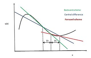
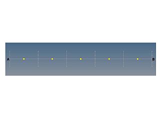
In applied mathematics, the central differencing scheme is a finite difference method that optimizes the approximation for the differential operator in the central node of the considered patch and provides numerical solutions to differential equations. It is one of the schemes used to solve the integrated convection–diffusion equation and to calculate the transported property Φ at the e and w faces, where e and w are short for east and west. The method's advantages are that it is easy to understand and implement, at least for simple material relations; and that its convergence rate is faster than some other finite differencing methods, such as forward and backward differencing. The right side of the convection-diffusion equation, which basically highlights the diffusion terms, can be represented using central difference approximation. To simplify the solution and analysis, linear interpolation can be used logically to compute the cell face values for the left side of this equation, which is nothing but the convective terms. Therefore, cell face values of property for a uniform grid can be written as:
Unsteady flows are characterized as flows in which the properties of the fluid are time dependent. It gets reflected in the governing equations as the time derivative of the properties are absent. For Studying Finite-volume method for unsteady flow there is some governing equations >
The upwind differencing scheme is a method used in numerical methods in computational fluid dynamics for convection–diffusion problems. This scheme is specific for Peclet number greater than 2 or less than −2
Finite volume method (FVM) is a numerical method. FVM in computational fluid dynamics is used to solve the partial differential equation which arises from the physical conservation law by using discretisation. Convection is always followed by diffusion and hence where convection is considered we have to consider combine effect of convection and diffusion. But in places where fluid flow plays a non-considerable role we can neglect the convective effect of the flow. In this case we have to consider more simplistic case of only diffusion. The general equation for steady convection-diffusion can be easily derived from the general transport equation for property by deleting transient.
The streamline upwind Petrov–Galerkin pressure-stabilizing Petrov–Galerkin formulation for incompressible Navier–Stokes equations can be used for finite element computations of high Reynolds number incompressible flow using equal order of finite element space by introducing additional stabilization terms in the Navier–Stokes Galerkin formulation.


